FLUX ROPES, TURBULENCE, AND COLLISIONLESS PERPENDICULAR SHOCK - PPPL Theory
←
→
Page content transcription
If your browser does not render page correctly, please read the page content below
FLUX ROPES,
TURBULENCE, AND
COLLISIONLESS
PERPENDICULAR SHOCK
WAVES: HIGH PLASMA BETA
CASE1
        G.P. Zank, M. Nakanotani, L.-L. Zhao,
                S. Du, & L. Adhikari
        Department of Space Science and Center for
          Space Plasma and Aeronomic Research
            University of Alabama in Huntsville

                                                     Photo by Shalom Jacobovitz / CC BY-SA 3.0

1Zank   et al., 2021, submitted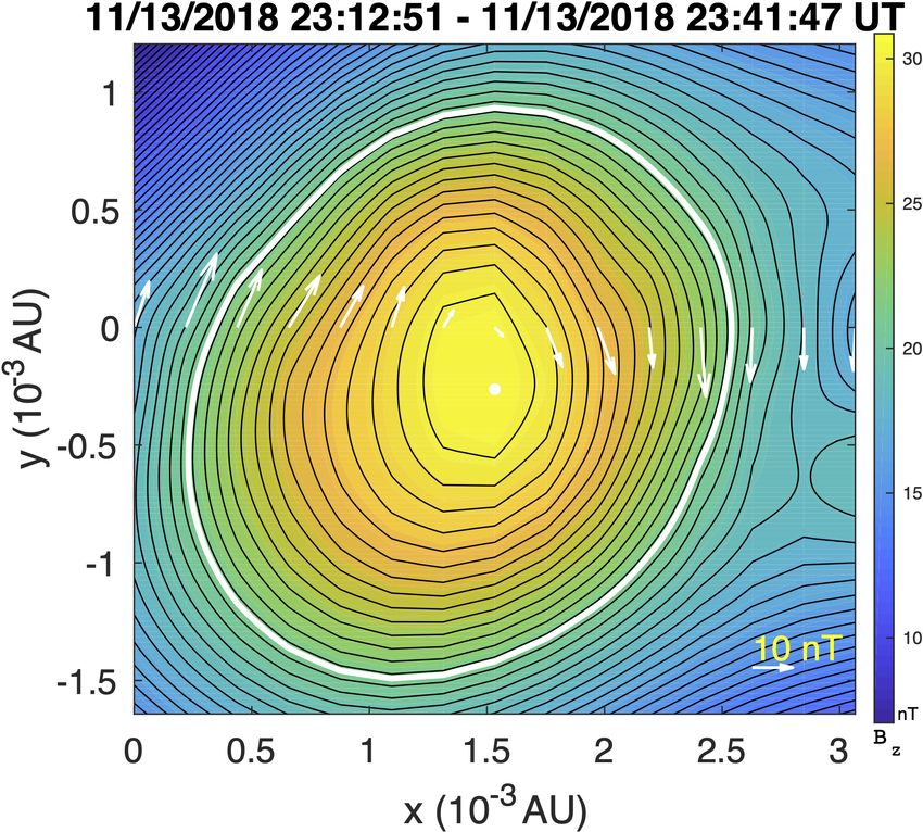
OUTLINE:

1) Motivation & Background: the transmission of fluctuations through boundaries and
   discontinuities

2) How does turbulence interact with shocks? Idealized theory and results

3) Comparison of (idealized) theory with heliospheric observations: Applicability of idealized
   theory for events at 1, 5, and 84 au, magnetic, kinetic energy, and density variance spectra

4) Concluding remarks

5) Some final thoughts about the evolution of turbulence behind a shock: simulations
1) Why the transmission of fluctuations through boundaries and
    discontinuities is interesting aka Motivation & Background
MOTIVATION 1)                       Burlaga et al. (2015, 2018)

Interval 1: Compressible turbulence with the fluctuating magnetic field almost entirely parallel to VLISM mean magnetic
field, and exhibiting ~k-5/3 spectrum in dB||
Interval 2: Incompressible turbulence almost exclusively, exhibiting ~k-5/3 spectrum in dB⏊ with same amplitude as dB||

These surprising observations raise three important questions:
i) What is the origin of the compressible fluctuations in the VLISM? and
ii) is the observed magnetic turbulence spectrum representative of interstellar turbulence in a partially ionized interstellar
     plasma, or is it somehow another manifestation of the mediation of the VLISM by heliospheric processes?
iii) Since fast magnetosonic waves can propagate further into the VLISM, why are these modes not seen in Interval 2?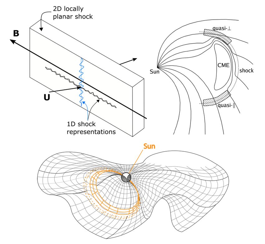
TD

    HTS                  ḆVLISM                                          Interval 1                           Interval 2
                 ḆIHS
                                  ẑ   ŷ
     ḆIMF

                                       x̂V1

             IHS

                                                                                                               Bow sh
                                                                                      B(
                                                                                        V
                                              Ḇ$        Ḇ#

                                                                                                                      ock/
            HP

                                                                                                                   wave
                                               x = Ψ(y,z,t)                                 V1

Ø IHS fast- and slow-mode waves incident on the HP generate only highly
                                                                                                   Subsonic
  oblique fast-mode waves that propagate into the VLISM.                                            VLISM
Ø VLISM fast-mode waves contribute magneKc fluctuaKons bz2 \neq 0 parallel to                     Incompressible
  the VLISM magneKc field and do not enhance the power in transverse modes                        MHD turbulence

Ø Fast magnetosonic waves undergo mode conversion via three-wave
  interacBon as they propagate in the homogeneous VLISM, decaying into an
  Alfvén wave and a zero-frequency Elsässer vortex, both of which possess
  only a transverse magneKc field component dB⏊. (Zank et al 2017, 2019)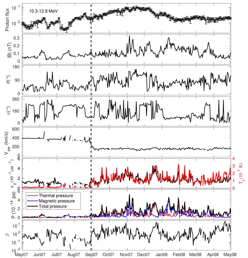
SOME BACKGROUND:
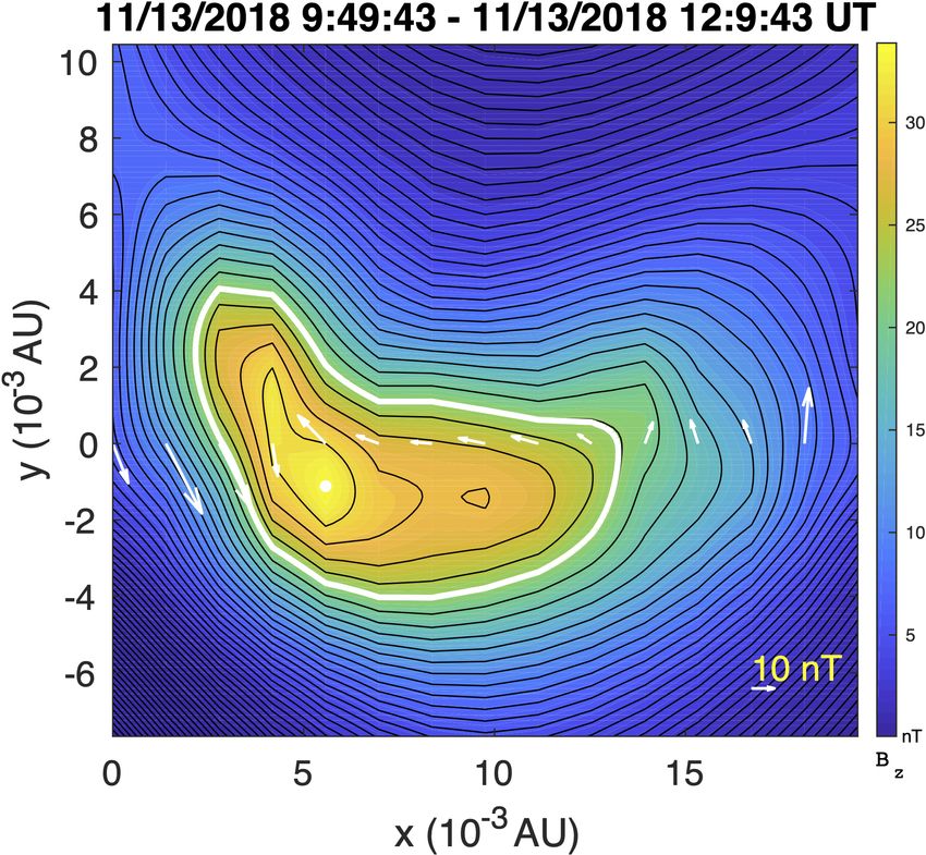
MAGNETIC FLUX ROPES
AKA MAGNETIC ISLANDS
Dura@on: 28.9 min
Scale size: 0.003 AU
Duration: ~ 140 min
Scale size: 0.0194 AU
Courtesy Roberto Bruno Zhao et al 2020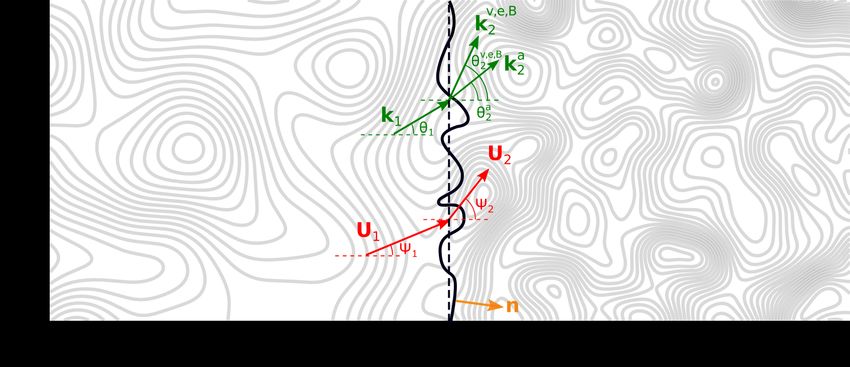
MoQvaQon 2): Zhao et al. 2018, 2019a. ApJ
Ulysses observaQons near 5 AU Flux enhancement downstream of the shock
Energetic proton flux
measured by Ulysses LEMS30
Magnetic field and plasma
parameters: (b) magnetic field
components and magnitude, (c)
proton speed and temperature,
(d) proton number density, and
(e) proton beta.
Ø During this period, Ulysses
crossed the heliographic
equator at 5.36 AU.
Ø A fast forward shock was
detected at 15:15:27 UT on
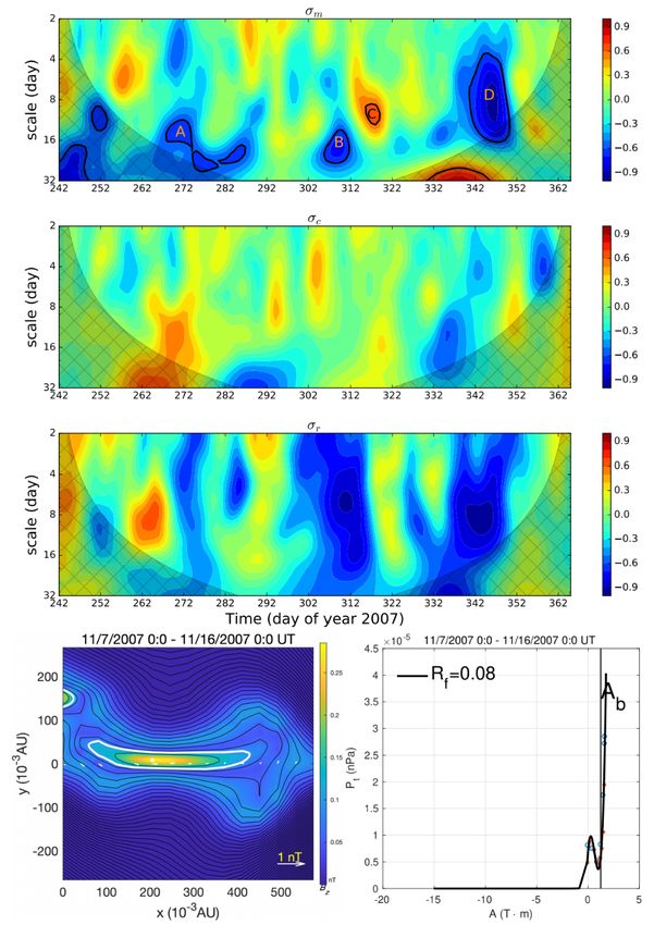
We automatically identify 31 magnetic flux rope structures 02/14/2004.
(grey shaded areas).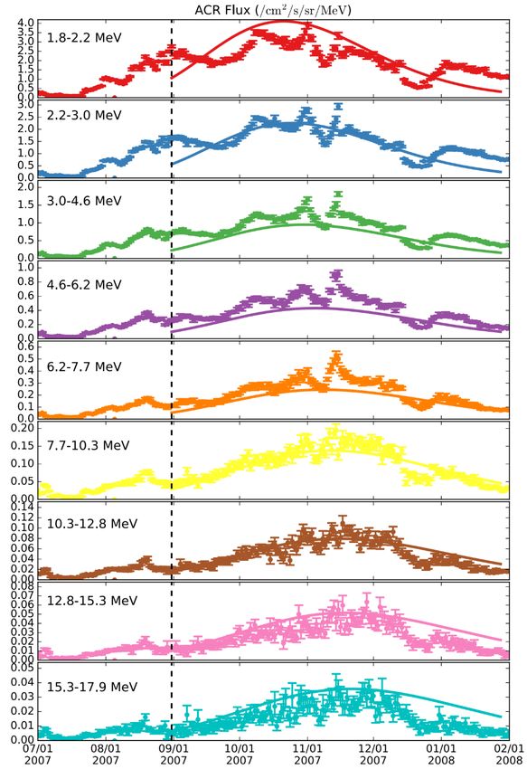
f(x)
Particle acceleration & SMFR

   Mean magnetic
   field

   Proton beta

                 Scale size
                               Stochastic acceleration by interacting magnetic
                               islands accounts successfully for the observed
                               energetic proton flux amplification (Zank et al.
                               2014, 2015; Zhao et al. 2018, 2019a).
Voyager 2 observaQon Zhao et al. 2019b. ApJ
ACR acceleration

Ø Observed ACR energeRc parRcle          f(x)
  spectrum ~ 100 days aTer the HTS
  crossing shows agreement with our
  reconnecRon-based stochasRc parRcle
  acceleraRon model (Zank et al. 2014,
  2015; Zhao et al. 2019b).
2) How does turbulence interact with shocks? Idealized theory and results1

1Zank   et al., 2021, submitted
2) How does turbulence interact with shocks (and discontinuities more generally)?
Classical problem
     Ø especially in gas dynamics, focus on the amplificaKon of sound (Burgers, 1946; Moore, 1954; Ribner 1954,+)
     Ø extended to MHD in 1960s (Kontorovich, 1959, +, good summary in Anderson, 1963), focus on amplificaKon of
        sound, but surprisingly done since then, and very liale done observaKonally.

    A somewhat systemaKc study iniKated by Pitna et al 2016, 2017, 2021 and Borovsky, 2020 but lacking in theoreKcal
    interpretaKon. The work presented here represents a first step in reexamining this classical problem.

    AmplificaKon of upstream spectrum and similarity of upstream and downstream spectra.

                                                                                                Pitna et al 2016, 2021
Ø Need to solve the time-dependent (non-conservation form of the) MHD equations on either side of the shock and then match the solutions across a free boundary (the shock). Ø We therefore need to derive the free boundary conditions. The shock surface and shock normal can be defined by
Ø Consider an upstream weak mean magneKc field B0 = B0z oriented perpendicularly to the flow vector U0 = (Ux, Uy, 0),
  such that transverse magneKc fluctuaKons (dBx, dBy, 0) are of the same order of magnitude as B0 and thus fluctuaKons
  dBz
Shock perturbed by a spectrum of small amplitude linearized fluctuations ⍺ exp [k.x – ⍵t] allows us to assume that

By way of example, focus on conservation of mass – fluctuating shock front yields R-H condition

Linearizing, applying assumpKons yields zeroth-order RH condiKons (perpendicular jump condiKons):

                                                                               (higher-order)
And the first-order equations for the shock front fluctuation, density, velocity, etc. amplitudes are given by:
Recall basic linear modes:
Transmission of incident vortical modes:
                                                     Rewrite all downstream variables in terms of the diverging fluctuations:

                                                      Ø To determine downstream angles for transmitted and generated
                                                        modes resulting from upstream vortical mode, we can assume that
                                                        the frequency ⍵ and tangential wave number ky are continuous
                                                        across the O(1) shock, i.e., ⍵1 = ⍵2 = ⍵ and ky1 = ky2 = ky.
                                                      Ø Solving ⍵’1 = 0 and either ⍵’2 = 0 (downstream vorticity or entropy
                                                        mode) or ⍵’2 = +/-a0k2 (downstream sound wave) yields angles for
                                                        transmitted/generated modes:

Notices that the downstream acoustic wave field is confined to propagation angles for which the discriminant is >= 0,
otherwise waves evanescent downstream. Slightly weaker condition holds:
FluctuaKng kineKc, density, and
magneKc energy amplificaKon
and spectra
amplitude
Ø Solutions to linearized b.c.’s for
the fluctuating velocity, density,
and magnetic field amplitudes as
functions of the incident flow
angle.
Ø Energies in the acoustic, vorticity,
ds2
entropic, and magnetic island
modes considered as separate
transmission problems for
upstream vorticity, entropy, and
du2
acoustic fluctuations.
Ø Consider two canonical cases that
resemble a high plasma beta
shock: a quasi-aligned case and a
quasi-perpendicular case in terms
of the incident flow vector.
dp2
Parameters ensures that both
shocks have the same compression
ratio r = 3.30.Velocity variance of transmitted fluctuations
vorticity
acous+c
Total kinetic energyDensity variance of transmitted fluctuations
entropy
acoustic
Total density varianceTransmission of upstream magnetic islands or flux ropes
Ø Magnetic modes fully decoupled from the gas
dynamic fluctuations in high plasma beta regime
Ø As before, ω1ʹ = 0 and ω2ʹ = 0, giving
Ø Downstream flux rope amplitude given by
where
Ø Amplification of magnetic islands relatively modest
but independent of shock obliquity.
Ø Transmission of an upstream spectrum of magnetic
island fluctuations with assumed spectral formDownstream spectra generated by incident vortical, entropy, and acoustic fluctuations:
1) For the upstream spectrum,
we prepare a number of
waves assuming omni-
direcKonal power spectrum
with θ1 randomly distributed
from 0 to π/2 (orange curve); Downstream Downstream Downstream kinetic
vortical velocity acoustical velocity energy spectrum
2) we calculate θ2 and the spectrum spectrum
amplitudes for each of the
vorKcal, entropy, and acousKc
modes transmiaed or
generated downstream for
each incident wave, and
3) we calculate the power
Downstream Downstream Downstream total
spectrum of the downstream entropic density acoustic density density spectrum
waves in k-θ2 space for each spectrum spectrum
of the generated modes and
then integrate over θ2 to
obtain the downstream omni- Incident spectrum of vortical modes
direcKonal power spectrum
(blue curve).Downstream Downstream Downstream kinetic
vortical velocity acoustical velocity energy spectrum
spectrum spectrum
Downstream Downstream Downstream total
entropic density acous+c density density spectrum
spectrum spectrum
Incident spectrum of entropy modesDownstream Downstream Downstream kinetic
vor+cal velocity acoustical velocity energy spectrum
spectrum spectrum
Downstream Downstream
Downstream total
entropic density acoustic density
density spectrum
spectrum spectrum
Incident spectrum of forward acoustic modes3) Comparison of (idealized) theory with heliospheric observations1 1Zank et al., 2021, submitted
3) Comparison of (idealized) theory with heliospheric observa:ons
            Consider 3 quasi-perpendicular shocks observed at 1 au (Wind), 5 au (Ulysses), and 84 au (Voyager 2)

Zhao et al. (2019a, 2019b)
investigated Ulysses and Voyager 2
events in context of magnetic flux
ropes that were identified
upstream and downstream of
shock
Are the assumptions inherent in theory consistent with observations?
1) Relative strength of fluctuating magnetic field to the upstream mean magnetic field: (1) Wind event: δB/B0 =
0.54 and δB⊥/B0 = 0.5; (2) Ulysses event: δB/B0 = 0.68 and δB⊥/B0 = 0.59, and (3) Voyager 2 event: δB/B0 = 12.47 and
δB⊥/B0 = 10.
ANS: B0 ∼ O(δB) is reasonable assumption for the three events. Values of the ratio δB⊥/B0 indicate most of power
resides in the 2D magnetic field fluctuations. Further confirmed by computing ⟨δB2D2 ⟩/⟨δBslab2 ⟩ and ⟨δU2D2 ⟩/⟨δUslab2 ⟩
upstream and downstream of each event finding values >> 1 [e.g., Wind: 23.76 (δB, up), 7.14 (δB, down), 15.96 (δU, up),
103.71 (δU, down)].
2) Plasma beta > 1?: Thermal pressure exceeds magneKc pressure for Wind and Ulysses shocks, so plasma beta ~1.5 to
3. EnergeKc parKcle pressure at HTS (anomalous cosmic rays, pickup ions) dominates upstream thermal and magneKc
field pressure e.g., Decker et al., 2008, implies plasma beta >> 1. ANS: Yes, beta > 1.
Based on Wind, Ulysses, and Voyager 2 parameters, the underlying assumptions in the analysis are met reasonably well and
can therefore compare the observed downstream spectra for the three shocks theoretical predictions with some confidence.Observed and predicted magnetic spectra Power spectrum analysis performed for each shock event using different Kme interval lengths, which represents roughly the inerKal range of turbulence at different radial distances. Observed upstream magneKc variance spectrum used for the source terms in theory. Comparison of the theoretical and observed downstream magnetic variance spectra for all three cases is excellent. Enhancement in downstream spectral intensity and the spectral slope well captured by theory with only noticeable discrepancy occurring in the dissipation range of the downstream Ulysses spectrum with some excess power.
Why should the transmission problem for magnetic turbulence agree so well with observations?

Ø Despite the idealized character of the theory and its restriction to magnetic islands, the reason for the good
  correspondence with the observed downstream PSDs likely stems from the two-component nature of solar wind
  turbulence.

Ø In this paradigm, for which there is both theoretical and observational support, solar wind turbulence is a
  superposition of a dominant quasi-2D component and a minority slab component (the quasi-2D-slab model of nearly
  incompressible (NI) MHD).

Ø The theory of turbulence transmission through a shock wave presented here describes the transmission of the
  dominant 2D component, and hence it is not altogether surprising that the theory accounts accurately for the
  observed downstream spectrum.
Observed and predicted kinetic energy and density spectra

Ø Only Wind plasma data of sufficient resoluKon
  used to determine kineKc energy and density
  variance spectra upstream and downstream of
  the shock.
Ø Unlike the magneKc variance case, we must
  consider source terms corresponding to
  incident vorKcal fluctuaKons, incident entropy
  fluctuaKons, and incident forward and
  backward acousKc fluctuaKons i.e., a
  superposiKon of the source terms.

 Ø Need the relative contribution of each observational mode to the kinetic energy and density spectra. The ratio of the
   2D to slab energy in velocity fluctuations for Wind is ⟨δU2D2⟩/⟨δUslab2⟩ = 15.96 ∼ 16. Use as proxy for energy in
   incompressible quasi-2D (vortical) and compressible (acoustic) fluctuations to decompose observed upstream kinetic
   energy and density variance spectra into vortical and acoustic kinetic modes and entropy and acoustic density
   fluctuations.
 Ø Thus, we assume that the upstream velocity and density fluctuations are primarily vortical and entropy
   (incompressible) modes instead of acoustic (compressible) modes. Consistent with the quasi-2D-slab superposition
   model.
4) Concluding remarks
Ø Despite the idealized formulaKon, we apply the theoreKcal shock-turbulence transmission problem to shocks
  observed at 1 au, 5 au, and 84 au. In each case, the ordering B0 ∼ O(δB) holds and fluctuaKng magneKc field
  component dominated by the δB⊥, validaKng the applicaKon of the theory to the observaKons.
Ø Since solar wind turbulence appears to be well described as a superposiKon of a dominant 2D component and a
  minority slab component, we consider the transmission of dominant quasi-2D turbulence across a shock while
  neglecKng the minority component.
Ø We took observed upstream magneKc spectrum and computed theoreKcal downstream spectrum and compared to
  observed downstream spectrum. Agreement between predicted and observed downstream magneKc variance
  spectrum remarkably good, matching spectral amplitude and spectral form and slope for all three cases.
Ø Only Wind shock had plasma data of sufficient resoluKon to allow comparison of observed and theoreKcal kineKc
  energy and density variance spectra.
Ø Observed Wind raKo of quasi-2D to slab energy moKvates decomposiKon of upstream fluctuaKons into primarily
  incompressible 2D modes, i.e., magneKc islands, vorKcal and entropy modes, and a smaller acousKc component.
Ø Complicated superposiKon of different downstream transmiaed and generated compressible and incompressible
  fluctuaKons yields the theoreKcally predicted spectrum that results in very saKsfying agreement with observaKons.

This gives us some confidence that
i) solar wind turbulence is comprised primarily of a majority quasi-2D component, and
ii) the linear free boundary theory presented here describes accurately the transmission of turbulence across
     collisionless quasi-perpendicular shocks.
Final thoughts if time permits
5) Some final thoughts about the evolution of turbulence behind a shock:

Pitna et al 2017 observations; Zank et al 2002 (simple) theory; Nakanotani et al 2020 simulations

                                                        Ø Decay of normalized kinetic (red crosses) and magnetic (blue
                                                          circles) energy behind interplanetary shocks (Pitna et al 2017,
                                                          superposed epoch analysis) plotted as function of nonlinear
                                                          time tnl.
                                                        Ø Averages show decreasing trends in both energies but trend not
                                                          monotonic – initial increase of both energies (up to tnl ~ 2),
                                                          constant value up to tnl ~ 10, followed by decay for larger times.
                                                        Ø Pitna et al consider model function form (Biskamp 2003)

                                                        Ø For magnetic energy decay, t0 = -4 +/- 2 and n = -1.2 +/- 0.1. For
                                                          kinetic energy decay, t0 = 0 +\- 2 and n = -1.2 +\- 0.1.

                                                        Ø Not unlike decay of turbulence behind grid in wind tunnel
                                                          experiments a la Batchelor.
NormalizaKon (Ek,0, Eb,0) immediately downstream
of the shock.
Nakanotani et al 2020: 2D Hybrid Simulation
Geometry and Parameters
Ø Force free condiKon Normalization
Ø Density and |B| is uniform • Length --> c/ωpi
• Time --> Ωi-1
⎡1
By = B0 tanh ⎢ cos
(
2π x + Vinj t ) ⎤⎥ , B = B sech ⎡⎢ 1 cos 2π ( x + V t ) ⎤⎥
inj • Velocity --> VA (Alfvén velocity)
⎢δ λ ⎥ z 0
⎢δ λ ⎥
⎣ ⎦ ⎣ ⎦
MA,inj 2
βi=βe 0.5
By, Bz
δ 0.1
λ 50 c/ωpi
ppc 100
Lx x Ly 200 x 204.8 c/ωpi
Δx=Δy 0.2 c/ωpi
Δt 0.01 Ωi-1
[Sironi & Spitkovsky, 2011, Burgess et al. 2016]Results: Animation of the Interaction of Current Sheets with a Shock Wave
Results: Snapshot of the Interaction of Current Sheets with a Shock Wave

             Ø Current sheets are compressed by the shock wave and become unstable downstream.
             Ø MagneKc fields become turbulent because of reconnecKon and the merging of islands

  T=80Ωi-1
Proton Energy Spectrum:
Ø Some protons are accelerated at the shock wave (blue line)
Ø Those accelerated protons are further energized due to reconnection events far downstream
Ø Black line shows the number of particles satisfying |v|>5VA.
Ø Flux increases as magnetic reconnection proceeds.
Nakanotani et al 2020
Ø Flux enhancement
responding to magnetic
reconnection activity
Ø Energetic particle Zhao et al. 2018, 2019a
profile similar to
predicted DSA-
reconnection transport
model [Zank et al.2015,
le Roux et al. 2015].You can also read