Food Security Dynamics in the United States: Insights using a New Measure
←
→
Page content transcription
If your browser does not render page correctly, please read the page content below
Food Security Dynamics in the United States:
              Insights using a New Measure∗
   Seungmin Lee†              Christopher B. Barrett†                 John F. Hoddinott†

                                        February 2021

                                             Abstract
       This paper introduces a new measure, the probability of food security (PFS), to study
       food security dynamics in the United States. PFS represents the estimated probability
       that a household’s food expenditures equal or exceed the minimum cost of a healthful
       diet, as reflected in the United States Department of Agriculture’s Thrifty Food Plan
       monthly cost estimates. PFS matches the official food security prevalence measure in
       a given period, but enables richer study of the dynamics and severity of food inse-
       curity. Applied to 2001-17 data from the Panel Study of Income Dynamics, we find
       that roughly half of households that become newly food insecure resume food security
       within two years. But the positive association of persistence with prior food insecurity
       means that half to two-thirds of food insecure households at any given time remain
       food insecure at least two years later. PFS varies dramatically with income and demo-
       graphic characteristics, such that inter-group prevalence and severity measures differ
       by one or two orders of magnitude. Households headed by non-White women with
       low educational attainment disproportionately suffer persistent, chronic food insecu-
       rity, while White-headed households without a college degree account for most of the
       business cycle-associated variation in national food insecurity.
   ∗
     We thank Liz Bageant, Anne Byrne, Will Davis, Matt Rabbitt and seminar participants at
Cornell, Mississippi State and USDA ERS for helpful discussions and comments on earlier drafts.
We are grateful to the US Department of Agriculture Economic Research Service (USDA ERS) and
the University of Kentucky Research Foundation for financial support through cooperative agreement
58-4000-6-0059 subaward 3200000900-20-212. The views expressed in this paper are the authors’
sole responsibility and do not represent those of USDA or ERS.
   †
     Charles H. Dyson School of Applied Economics and Management, Cornell University

                                                  1
1 Introduction
Food security means that people have access at all times to sufficient and
nutritious foods to enjoy an active and healthy life (FAO 2020; Coleman-Jensen et
al. 2020). Food insecurity has well-established, long-term, negative implications for
health and educational outcomes, social skills, and adult economic productivity (Jy-
oti, Frongillo, and Jones 2005; Alderman, Hoddinott, and Kinsey 2006; Hoddinott
et al. 2008; Gundersen and Ziliak 2015; Gundersen and Kreider 2009; Hoddinott et
al. 2013) and therefore has been an important policy objective globally.
In the United States (US), at least one out of ten households has been food
insecure in any given year since the United State Department of Agriculture (USDA)
first began reporting the current official food security measure in 1995. The most re-
cent, 2019 nationwide prevalence for the US was 10.5% (Coleman-Jensen et al. 2020).
But the Coronavirus Disease (COVID) pandemic shock has driven this sharply higher
(Schanzenbach and Pitts 2020). According to the Census Bureau’s Household Pulse
Survey for Nov. 25 - Dec. 7, 2020, roughly 13 % of adults reported their households
did not have enough to eat in the prior week, nearly four times the rate rate that
USDA had reported for the whole of calendar year 2019 (Center on Budget and Policy
Priorities 2021).
Given food insecurity’s adverse effects on a host of economic, health and social
outcomes, and those outcomes’ feedback on household incomes, dietary behaviors, and
subsequent food security status, a sound descriptive understanding of food security
dynamics can help with effective policy design and evaluation. For example, if one
expects the millions of households unexpectedly driven into food insecurity by the
2020 COVID shock to quickly become food secure again, temporary private and
public food assistance financed by one-off appropriations or charitable donations may
suffice to avert longer-term consequences. If instead one should reasonably expect a
large share of the suddenly food insecure to persist in that new (to them) state, longer-
lasting interventions and funding arrangements may be necessary. And if identifiable
subpopulations predictably experience different food security dynamics, that should
inform program targeting. Unfortunately, the empirical literature on food security
dynamics in the US is quite thin, arguably insufficient to provide a firm empirical
foundation to inform policy.
2The dearth of food security dynamics evidence stems directly from measure-
ment and data collection issues that are global, not specific to the US (Barrett
2010). US food security studies rely mainly on the Household Food Security Measure
(HFSM), the official measure developed by USDA based on a survey instrument first
introduced in the Household Food Security Survey Module (HFSSM) supplement to
the Current Population Survey (CPS) in 1995. Households answer up to 18 HFSSM
questions (10 questions for households without children) listed in Table A1. House-
hold food security status is then assessed based on the number of questions households
affirm, standardized into 29 discrete values in the [0.0,9.3] interval and three ordinal
categories (food security, low food security, and very low food insecurity) to enable
comparison among households with and without children (Table A2).The CPS has a
rotating panel design that tracks the same household no more than 8 times over a
16-month period, including a maximum of two observations from the annual HFSSM.
So CPS does not enable the study of household food security dynamics beyond a one
year interval.
Other longitudinal household surveys have fielded the HFSSM among the same
households for longer intervals, but even those data sharply limit the study of food
security dynamics. The Panel Study of Income Dynamics (PSID) has implemented
HFSSM only for five waves (1999, 2001, 2003, 2015, 2017), within which there exists
a significant gap from 2003-15. The Early Childhood Longitudinal Survey (ECLS)
collected food security data over different survey periods (1999-2007, 2010-2016). But
both surveys span less than 10 years, do not include the full HFSSM in most waves,
and their samples are restricted to households with young children, thus they are not
nationally representative.
The discrete, ordinal nature of the HFSM also limits our capacity to under-
stand change in food security status over time as one might with a continuous measure.
For example, for households with children who affirm every question in consecutive
periods, the measure provides no additional information regarding prospective change
in the severity of their food insecurity (Bickel et al. 2000). The official categories are
also quite broad and invariant with respect to the specific manifestation of com-
promised food access. Each household with children that affirms any eight (of 18)
questions is similarly classified as suffering very low food security. But just as pol-
icymakers now routinely rely on poverty measures in the Foster–Greer–Thorbecke
3(FGT, Foster, Greer, and Thorbecke 1984) tradition that can report more than just
headcount prevalence, enabling study of distribution-sensitive severity of deprivation,
so too would it be nice to study fluctuations in food insecurity severity over time.
These data limitations have significantly limited research on food security dy-
namics in the US. A few nice studies investigate household-level dynamics over time
(Hofferth 2004, Kennedy et al. 2013, Ryu and Bartfeld 2012, Wilde, Nord, and Zager
2010). But none has more than five observations per household, making analysis
of dynamics somewhat vulnerable to both measurement error and real, but transi-
tory shocks to food security status (Baulch and Hoddinott 2000; Dercon and Shapiro
2007; Naschold and Barrett 2011). Prior studies can also only study transitions and
persistence using discrete categorical status, necessarily suppressing within-category
variation over time in the severity of the food insecurity households experience. Fur-
ther, these prior studies all predate Great Recession, raising questions as to past
findings’ current relevance.
To overcome these limitations, we introduce a new measure that is directly
linked to the official HFSM and is implementable in longer panels, such as PSID,
that include continuous measures of food expenditures. The probability of food secu-
rity (PFS) is the estimated probability that a household’s observed food expenditures
equal or exceed the minimal cost of a healthful diet, as reflected by the USDA’s Thrifty
Food Plan (TFP) cost that provides the basis for maximum Supplemental Nutrition
Assistance Program (SNAP) allotments. We estimate PFS by computing the con-
ditional density of household food expenditures and estimating, for each household
and survey period, the inverse cumulative density beyond the TFP threshold spe-
cific to that household composition and survey date. PFS adapts an econometric
method (Cissé and Barrett 2018) that has been applied to study food security in
the low-income world (Upton, Cissé, and Barrett 2016; Phadera et al. 2019; Vaitla
et al. 2020; Knippenberg, Jensen, and Constas 2019).
The PFS measure enables the study of food security dynamics in longer panels
than has been previously feasible because food expenditures data are more commonly
available in each survey wave in longitudinal household surveys than are HFSSM-
based measures. Because PFS is a continuous, decomposable measure in the FGT
tradition, it also enables the study of distribution-sensitive measures of food security
severity, including at sub-group level. PFS thus offers the opportunity to obviate the
4data constraints that have previously limited the study of food security dynamics.
We apply the new PFS measure to investigate household-level food security
dynamics in the US over 17 years using PSID data. We use approximately 23,000
survey responses from 2,700 nationally representative households surveyed biennially
from 2001 to 2017, nine times each in total. We employ two different approaches to
study food security dynamics reflected in PFS: a spells approach to study transitions
in food security status between survey waves, and decomposition into chronic and
transitory food insecurity based on 17-year, household-specific histories. We estimate
these measures nationally but also by subgroups based on household characteristics
such as the gender, race and educational attainment of the household head.
The descriptive insights afforded by this new measure are striking. We find
that roughly half of households that newly become food insecure in a given year
become food secure within two years. The persistence of food insecurity is positively
correlated with the duration of the household’s prior food insecurity experience. As
a result of these two facts, on average from half to two-thirds of households that
are food insecure in any given year will still be food insecure two years later. The
duration households remain food insecure is negatively correlated with the strength of
the macroeconomy. During the Great Recession, for example, recovery from new food
insecurity episodes slowed markedly relative to before the macroeconomic slowdown,
or as compared to later in the 2010s. At sub-group level, the persistence of food
insecurity is strongly associated with household characteristics. Food security status
varies largely by demographic characteristics and, especially, household income, and
relatively less by geography. Headcount prevalence rates differing by a factor of up
to 28 - and severity measures by a factor of up to 112 - among sub-groups defined by
race, gender and educational attainment.
The result is a mosaic of distinct patterns of food security dynamics in the
US. Black and female-headed households with low educational attainment dispropor-
tionately suffer persistent, chronic food insecurity, while household headed by White
men with a college education hardly ever suffer food insecurity, and a majority of the
intertemporal fluctuation in food security status occurs among White-headed house-
holds without a college degree. The latter group accounted for 81% of the surge in
food insecurity from 2007 to 2009, for example. This new descriptive evidence opens
up many deeper questions about underlying mechanisms, the causal impacts of food
5assistance and other interventions, etc. The PFS measure offers a useful tool with
which the research and policy communities can begin to explore these issues.
2 Empirical Framework
2.1 Data
This study uses the PSID, the leading nationally representative panel survey
of US households, for two reasons. First, the PSID included the HFSSM in the 1999-
2003 and 2015-2017 waves,1 enabling us to calibrate and validate the PFS measure
against the official food security measure that USDA estimates from CPS data each
year. Second,the PSID’s intensive tracking of a nationally representative sample of
US households annually from 1968-1997 and biennially since 1997, enables study of
long-term dynamics in a way no other data set does.2 .
We study a balanced sample of approximately 23,000 observations from 2,700
households where household heads remain the same over the 9 waves from 2001 to
2017. 3 The PSID has three sub-samples; Survey Research Center (SRC), which is
1. There are minor differences in the food security module between the PSID and the CPS.
For example, while the CPS includes household income level as a screening criterion for whether
households answer the HFSSM, the PSID does not have any screening criteria and all households
answer the HFSSM instead. Tiehen, Vaughn, and Ziliak (2019) explains the differences in detail,
concluding that their findings “lend credence to the use of the PSID for food insecurity research”
(p.20).
2. The PSID has regularly adjusted its survey weights to account for differential attrition rates
and family composition change, and added a new, nationally representative immigrant population
subsample to maintain its representativeness. As a result, economic indicators estimated from the
PSID either align fairly closely with, or at least exhibit similar trends as, those derived from other
representative surveys such as the CPS or the Consumer Expenditure Survey (Andreski et al. 2014;
Li et al. 2010; Gouskova, Andreski, and Schoeni 2010; Tiehen, Vaughn, and Ziliak 2019)
3. We omit attrited and split-off units (i.e., those that disappear from the sample or newly created
households from existing households), for the following reasons. First, they necessarily offer shorter
sequences of observations, which can improve precision in understanding shorter-term dynamics but
much less so on the longer-term dynamics that motivate this paper. Second, PSID survey weights
update regularly to adjust for panel attrition due to non-response (Chang et al. 2019). Third, split-
off households may still depend heavily on their origin households, leading to complex correlation
structures in the data that could bias descriptive statistics.
6the original nationally representative household sample, Survey of Economic Oppor-
tunities (SEO), which is an over-sampling of low-income households so as to permit
the study of that subpopulation, and Immigrant Refreshers added in 1997, 1999 and
2017 to represent immigrant population. We use the SRC and SEO subsamples,
which account for 93% of the entire PSID population. We omit the immigrant sub-
sample because its representativeness with respect to food security status has not yet
been validated, unlike the other two sub-samples (Tiehen, Vaughn, and Ziliak 2019).
Table 1 reports summary statistics of the sample households and each sub-sample4 .
Table A3 describes the variables used in this paper. As one would expect from the
over-sampling design of the SEO sub-sample, SRC households have higher per capita
income and food expenditures, are more educated and less likely to receive food stamp
assistance in the previous year, as compared to the SEO households. Note that the
income variable does not include the value of food stamps or other public benefits
(e.g., free or reduced price school meals).
The probability of food security (PFS) measure provides an estimate of the like-
lihood that a household’s food expenditures equal or exceed some normative threshold
value. Households report three different food expenditure categories - at home, deliv-
ered and eaten out - with their choice of period from daily to yearly. During our study
period majority of households reported weekly expenditure.5 PSID has provided the
annual food expenditure by imputing and aggregating the three food expenditures
since 1999. A natural candidate threshold is the cost of the USDA’s Thrifty Food
Plan (TFP) diet, which “serves as a national standard for a nutritious, minimal-
cost diet” (Coleman-Jensen et al. 2020). USDA reports TFP monthly in its Cost
of Food Reports.6 The report provides individual costs per gender and age group as
well as multipliers for different household sizes. We generate household-year-specific
TFP diet costs by matching individual household member’s age and gender with the
4. Unless expressly indicated, all parameter estimates and standard errors we report are adjusted
to account for panel survey data structure based on the survey weights, stratum and cluster codes
the PSID includes in its raw data. We constructed a new survey weight and a new cluster to take into
account serial correlation within household, as suggested by Heeringa, West, and Berglund (2010).
5. In the entire 1999 wave 83% of households reported weekly at-home food expenditure
6. The Cost of Food Reports present weekly and monthly costs corresponding to four USDA-
designed food plans: Thrifty, Low-cost, Medium-cost, and Liberal. TFP is the cheapest of these. It
is used to determine a household’s maximum SNAP benefit (Ziliak 2016).
7Table 1: Summary Statistics
Total SRC SEO
mean sd mean sd mean sd
Household Head
Age 56.35 13.62 56.58 12.17 53.19 23.84
Race
White 0.85 0.35 0.91 0.24 0.01 0.20
Non-white 0.15 0.35 0.09 0.24 0.99 0.20
Married 0.61 0.48 0.63 0.42 0.30 0.90
Female 0.22 0.41 0.20 0.35 0.50 0.98
Highest educational degree
Less than high school 0.11 0.31 0.10 0.26 0.24 0.84
High school 0.27 0.44 0.27 0.39 0.35 0.93
Some college 0.25 0.43 0.25 0.38 0.27 0.87
College 0.37 0.48 0.39 0.43 0.14 0.68
Employed 0.65 0.47 0.66 0.42 0.58 0.97
Disabled 0.19 0.39 0.19 0.34 0.23 0.83
Household
Income per capita 40.26 30.43 41.60 27.30 21.71 35.24
Food expenditure per capita 3.65 2.11 3.73 1.87 2.51 3.55
Family size 2.22 1.16 2.22 1.02 2.26 2.67
% of children 0.10 0.19 0.10 0.17 0.16 0.47
Food Assistance
Food stamp 0.05 0.22 0.04 0.18 0.22 0.81
Child meal 0.04 0.19 0.03 0.15 0.18 0.75
WIC 0.01 0.11 0.01 0.08 0.05 0.42
Elderly meal 0.01 0.07 0.00 0.06 0.02 0.24
Change in status
No longer employed 0.08 0.27 0.08 0.23 0.10 0.58
No longer married 0.01 0.11 0.01 0.10 0.01 0.19
No longer owns house 0.03 0.16 0.03 0.14 0.03 0.33
Became disabled 0.07 0.26 0.07 0.23 0.07 0.51
N 22,556 16,602 5,954
Note: The sample consists of the households from the SRC and the SEO sample surveyed
from 2001 to 2017. Top 1% values of income and expenditure values are winsorized.
8monthly costs reported in June of each year, summing up the individual costs within
household and applying the appropriate multiplier corresponding to the household
size, and then dividing by the number of household members in order to express
everything in per capita terms.7
2.2 Empirical Strategy
2.2.1 Construction of the PFS
We construct the PFS following the general method introduced by Cissé and
Barrett (2018). First, we estimate the conditional mean of household per capita
food expenditures by regressing it on a polynomial of its prior period value - thereby
allowing for the possibility of nonlinear dynamics - and other covariates.
3
X γ
Wijt = βMγ Wijt−1 + δM Xijt + ωM t + θM j + uM ijt (1)
γ=1
In equation 1, Wijt is annual per capita food expenditures for household i in state
j and year t. We construct this dependent variable by dividing the annual food
expenditure by the number of members of the household. Note that food expenditures
does not include the value of government transfers such as food stamps received. Food
expenditures have long been used in food security analysis internationally not only
because they direct capture household food consumption but also because they are
strongly associated with other food security indicators, such as dietary diversity, food
consumption scores, coping strategy indices, etc.(Hoddinott and Yohannes 2002).
Xi,t is a vector of household-level covariates that the existing literature has
found associated with food security, including demographics (age, gender, race, and
educational attainment of the household head), income (which does not include the
value of government transfers, such as SNAP), and changes since the prior survey
round in employment, marriage, housing and disability status. The ωt and θj pa-
rameters are year- and region- fixed effects and the M subscript indicates parameters
7. For households in Alaska and Hawaii where costs are only reported semi-annually, we use the
costs reported in the first half of the year. Also, those two states do not report the costs for some
age groups (1-5, 12-19, 51+ years). So we use the costs reported for 6-8 for the first missing group
and the costs reported for 20-50 for the other two missing groups.
9related to the (conditional) mean. We include the lagged dependent variable up to a
third order polynomial in Wijt .8 The predicted value of the outcome variable, Ŵijt , is
the conditional mean of the household per capita food expenditure distribution. We
assume Wijt follows a Gamma distribution since it is continuous and non-negative.9
We therefore estimate a generalized linear model (GLM) logit link regression for
equation 1.
Given a mean zero error term, E[uM ijt ] = 0, the expected value of the squared
residuals, E[û2M it ], equals the conditional variance. So regressing the squared resid-
uals from the conditional mean equation on covariates yields a regression equation
for the conditional variance of per capita food expenditures, using the same basic
specification as in equation 1:
3
X γ
(ûM it − E[ûM it ])2 = û2M it = βVγ Wijt−1 + δV Xijt + ωV t + θV j + uV ijt (2)
γ=1
where the V subscript stands for (conditional) variance and the other notation is as
in equation 1. We estimate the conditional variance equation 2 by ordinary least
squares because GLM would not reliably converge.
The final step uses the household-and-period-specific conditional mean and
variance estimates to construct a household-and-period-specific cumulative density
function (CDF). Assuming Wijt ∼ Gamma (α, β), we calibrate
the parameters using
2
Ŵijt 2
σ̂ijt
the method of moments such that α= 2
σ̂ijt
,β = Wijt
where Wijt is the per capita
cost of the TFP diet calculated as described in Section 2.1.10
We then estimate the probability of food security (PFS) as the inverse CDF,
i.e., the conditional cumulative density above the household-specific TFP diet cost,
ρ̂ijt = 1 − F Xijt , Wijt−1 |Wijt ∈ [0, 1] . (3)
8. Table A4 shows that the coefficient estimates on higher order polynomial terms are statistically
insignificant thus the principle of parsimony favors a third order polynomial. That decision is
supported by Akaike Information Criterion (AIC) statistics that remain nearly unchanged across
different polynomial specifications.
9. The mean of the outcome differs significantly from its variance in our sample, so we do not use
a Poisson distribution, which requires the mean equals the variance.
10. For 847 observations (3.7% of the sample) the conditional mean and/or variance estimates
were negative, thus their inverse CDF could not be constructed.We drop those outliers from the
subsequent analysis.
10We then categorize households as food secure in year t if ρ̂it ≥ Pt , where Pt is the
externally determined cut-off probability such that the proportion of food secure
households in year t matches the annual USDA population prevalence estimate. For
example, if the USDA reported 10% of households as food insecure in year t, then we
sort households in year t by the PFS and assign the PFS of the household at 10th
percentile in the weighted sample as Pt .11 The estimated prevalence of food insecure
households is thus mechanically equal to the official USDA estimate.
We validate the PFS as a food security measure as follows. First, we assess
how strongly PFS correlates with the HFSM both by estimating rank correlations and
by regressing the HFSM on the PFS measure. Second, we regress both the official
USDA and the PFS measures on household characteristics and examine whether the
two different measures exhibit similar associations with covariates.
2.2.2 Household-level Dynamics
Reliably distinguishing chronic from transient food security is essential to in-
form policy design. Perhaps especially now, in the wake of 2020’s massive unem-
ployment shocks due to the COVID pandemic and its economic disruptions, there is
considerable value in having a clear sense as to how long one might expect households
suddenly thrust into food insecurity to persist in that state, at least absent interven-
tions to ameliorate their situation. Does job loss lead to similar near- or long-term
food insecurity as does a lasting physical or mental disability caused by the disease,
or sudden homeless following an eviction or foreclosure after one cannot keep up with
housing payments? If some identifiable subpopulations are much more likely to suffer
persistent food insecurity than others, it may be feasible to target such people for
programs intended to remedy a longer-term challenge while encouraging shorter-term
safety net protections for those expected to escape food insecurity almost as quickly
as they entered. The longer panels we can build with PFS, as compared to the official
measure based on HFSSM data, permits more careful study of food security dynamics
that might usefully inform policy design and evaluation.
11. An alternative approach would be using a fixed cut-off probability P over the period as Cissé
and Barrett (2018) originally did. We use varying cut-off probabilities so as to ensure our analysis
corresponds directly with the official HFSM. Figure A1 depicts the resulting interannual variation
in Pt , which varies between (0.48, 0.59).
11Figure 1: Food Security Transition Matrix
We adopt two different approaches to study food insecurity dynamics, borrow-
ing from the poverty dynamics literature. The spells approach studies the duration
of households’ continuous experience of food insecurity, as reflected by households’
PFS in successive survey waves. We categorize observations into four categories: (1)
Food insecure in two successive waves, (2) Food insecure in the preceding wave but
food secure subsequently, (3) Food secure in the preceding wave but food insecure
subsequently, and (4) Food secure in both waves. Figure 1 depicts this categorization.
This joint distribution naturally yields estimates of persistence and entry rates.
The persistence rate is the conditional probability that a food insecure household
remains food insecure the next survey wave. One minus the persistence rate is often
called the exit rate. The entry rate is the conditional probability a household becomes
food insecure in the following wave conditional on being food secure initially. Under
the spells approach, we classify food insecurity as recurrent if it persists for two or
more consecutive waves and transient if it is not observed in consecutive survey waves.
We can compute persistence and entry or exit rates for distinct sub-populations in
order to investigate inter-group heterogeneity in food security dynamics. We can
also investigate the distribution of spell lengths - i.e., of duration of consecutive
observations of food insecurity - as well as spell lengths and exit rates conditional on
a household newly entering the ranks of the food insecure. These estimates help us
understand whether food security exhibits path dependence, unconditionally or for
distinct sub-populations.
12The second, permanent approach to studying food security dynamics identifies
chronic food insecurity by mean intertemporal PFS and transient food insecurity
by deviations from the household-specific intertemporal mean. Following Jalan and
Ravallion (2000) denote T F Ii as the observed sequence of PFS measures for household
i and CF Ii as its chronic component, thus the difference, T F Ii − CF Ii , represents
the transient component:
T
!α
1X min(P F Sit , Pt )
T F Ii (α, P F Si1 , ..., P F Sit ) = 1− (4)
T t=1 Pt
" P # α
T
t=1 P F Sit
CF Ii (α, P F Si1 , ..., P F Sit ) = 1 − min 1, P T
(5)
t=1 Pt
A household with CF Ii > 0 is chronically food insecure under the permanent
approach, i.e., in expectation it is food insecure in any given period. TFI and the CFI
are FGT-style measures, with important modification that they aggregate over time
within households while FGT indices aggregate over households within a specific
time period. The aversion parameter α reflects sensitivity to the severity of PFS
shortfalls relative to Pt . For α = 0, 1, 2, CF Ii reflects the frequency of food insecurity,
average severity of such shortfalls, which we lable the food insecurity gap (FIG), and a
more loss-averse, squared food insecurity gap (SFIG), respectively. TFI is additively
decomposable into sub-periods; the TFI over any period is simply the weighted sum of
TFI over the component sub-periods.12 In order to reduce measurement and sampling
error, we compute TFI and CFI only for the 99% of sample households with five or
more years of non-missing PFS.
We again categorize households into four categories, but now based on the
permanent approach’s CF Ii and T F Ii measures rather the spells approach. The first
12. As a FGT-style measure, TFI satisfies Sen (1976)’s monotonocity and transfer axioms between
time periods. The monotonicity axiom means that TFI falls weakly monotonically with an increase
in PFS, while the transfer axiom means that TFI falls as a household transfers food expenditures
from a higher PFS period to a lower one. See Foster, Greer, and Thorbecke (1984) or Cissé and
Barrett (2018) for more in depth discussion and proofs. CFI, however, satisfies the monotonicity
axiom but neither satisfies the transfer axiom nor is it additively decomposable into sub-periods
because it takes as an argument the intertemporal mean PFS, which cannot be decomposed into
sub-periods, as Calvo and Dercon (2007) explain.
13category are persistently food insecure households, i.e., CF Ii > 0 and P F Sit < Pt ∀t.
The second category encompasses households that are chronically but not persistently
food insecure, i.e., CF Ii > 0 and ∃t such that P F Sit ≥ Pt . The third category are
transiently food insecure households, i.e., CF Ii = 0 and ∃t such that P F Sit < Pt .
Finally, there are persistently food secure households, i.e., CF Ii = T F Ii = 0.
The two methods overlap imperfectly. The recurrently food insecure under the
spells approach include the persistently food insecure under the permanent approach
as a proper subset. The former could include some households that the permanent
approach classifies as chronically but not persistently food insecure because those
identified as chronically food secure by the spells approach can experience transient
food security in a given year. Conversely, the persistently food secure under the
permanent approach include as a proper subset the recurrently food secure under the
spells approach, i.e., those who never experience consecutive periods of food insecurity
but could experience nonconsecutive periods of food insecurity.
Each method has both strengths and weaknesses. Lawson and McKay (2002)
favors the permanent approach not only because it is less vulnerable to measurement
error and data truncation - i.e., data unavailable prior to the start year and after the
final year of the study period can censor spell length observations - but also when
survey intervals are more than a year in length, because one cannot observe possible
breaks in a spell during multi-year, inter-wave intervals. The permanent approach,
however, assumes a stationary process - i.e., it ignores trends or permanent shocks
that lead to a structural change over time - and requires longer periods of panel data
in order to estimate the intertemporal mean without small sample bias.
2.2.3 Groupwise aggregation
One can aggregate PFS over households - or, equivalently, decompose population-
level PFS - to generate group-specific estimates and track how those change over time.
We construct three different FGT-style national indices for each time period t based
on the same α aversion parameter introduced in equations 4 and 5 and each house-
hold’s PFS estimate: the prevalence or headcount ratio (HCR), the food insecurity
gap (FIG) and the squared food insecurity gap (SFIG):
14N
!α
1 X min(P F Sit , Pt )
F GTt (α, P F S1t , ..., P F SN t ) = 1− (6)
N i=1 Pt
where α is the aversion parameter, N is the number of households in the population
and Pt is the threshold probability of food security from Section 2.2.1. HCR, FIG
and SFIG take α = 0, 1, 2, respectively, and are thus also referred as P0 , P1 and
P2 measure. The HCR represents the proportion of food insecure households in the
population. The FIG, analogous to the poverty gap measure in poverty literature,
describes the depth of food insecurity and can be interpreted as the average PFS
shortfall of the population. For instance, if FIG is x%, then household-average PFS
in the population is lower than the threshold PFS by x%. The SFIG, analogous to the
squared poverty gap index in poverty literature, describes the severity of food inse-
curity where the (normalized) gap between the PFS and its cut-off value is weighted
by itself.
These measures complement each other, each having both strengths and weak-
nesses. On one hand, the HCR is the simplest and the most intuitive among the three
measures. The official USDA-reported food security prevalence measure is an HCR.
On the other hand, the HCR satisfies neither of Sen (1976)’s two basic axioms of
well-being measures: the Monotonicity Axiom, which requires a measure increase as
the food security of any person declines, and the Transfer Axiom, which requires the
measure increase if there is a transfer from someone who is food insecure to someone
whose is less (or not) food insecure. On the other hand, the FIG and the SFIG are
less intuitive, but the FIG satisfies the Monotonicity Axiom (but not the Transfer
Axiom), while the SFIG satisfies both axioms. For that reason, we favor the more
distribution-sensitive SFIG measure in reporting on severity of food insecurity.
We report HCR, FIG and SFIG measures overall over the study period, 2001-
17. Since all three measures are additively decomposable, we decompose these mea-
sures and their intertemporal patterns into groupwise aggregates based on key, easily
targetable attributes of a household head: race, gender and education. This allows us
to unpack whether different groups experience chronic and transitory food insecurity,
or food insecurity prevalence and severity, differently.
153 Results
3.1 Validating the PFS measure
We begin by confirming the correspondence of the PFS measure with the
official USDA Household Food Security Measure (HFSM). We re-scaled the HFSM
such that it varies from zero to 1 and higher scale implies higher food security13 ,
so we can compare it with the PFS. The conditional mean and variance regression
coefficient estimates from equations (1) and (2) are reported in Table A5. Both
conditional moments are significantly nonlinear in lagged per capita food expenditures
and in the age of household head. The basic patterns of associations are intuitive:
food expenditures are positively correlated with income, educational attainment, and
employment status, and negatively correlated with family size, a female household
head, and among SNAP and WIC recipients. These associations suggest PFS relates
to household attributes in a sensible way.
The PFS measure is strongly, positively correlated with the USDA scale. The
Spearman rank correlation coefficient and Kendall’s τ between the two measures
are 0.31 and 0.25, respectively, significantly different from zero. The regression of
the USDA scale on the PFS – reported in Table 2 – shows a strongly significant
positive relationship despite the fractional nature of the HFSM and both measures’
strong positive skewness.14 By the nature of its construction, the PFS distribution
is relatively smooth as compared to the HFSM, resulting in an association that is
stronger over the lower range of the PFS, that is, among the food insecure, where we
most want the measures to correspond.
Table 3 shows how household characteristics associate with the USDA scale
and the PFS. In column (1) and (2), correlates that are statistically significantly as-
sociated with both the USDA scale and the PFS, and with the same sign, include
income per capita, % of household members who are children, receipt of food stamps,
lack of a high school diploma, and disability status, where the first two are positively
and the other three are negatively associated. Most covariates have the same sign es-
13. HF SMrescale = 9.3−HF9.3
SM
14. Among the PSID sample households, 89% have a USDA scale value of 1, indicating food
security, while the median estimated PFS is 0.9 and the 90th percentile equals 0.996). Figure A2
displays these distributions.
16Table 2: Regression of the USDA scale on the PFS
(1) (2) (3) (4)
HFSM HFSM HFSM HFSM
PFS 0.180∗∗∗ 0.465∗∗∗ 0.182∗∗∗ 0.442∗∗∗
(0.02) (0.08) (0.02) (0.08)
PFS2 -0.217∗∗∗ -0.199∗∗∗
(0.05) (0.05)
Fixed Effects N N Y Y
N 11,798 11,798 11,798 11,798
R2 0.117 0.127 0.137 0.146
∗ p < 0.10, ∗∗ p < 0.05, ∗∗∗ p < 0.01
Note: Sample include households surveyed in 2001, 2003, 2015 and 2017 with
both the USDA scale and the PFS available. Fixed effects include region (state)
and time (wave) fixed effects.
timates, even if the magnitudes and precision of the estimated coefficients differ. The
PFS’ correlations with these variables generally conform with the existing literature
(e.g., Hofferth 2004, Tiehen, Vaughn, and Ziliak 2019). There exist a few correlates,
however, that significantly correlate with both the USDA scale and the PFS, but
in opposite directions. For example, age is associated convexly with the HFSM but
concavely with the PFS. To us, the PFS relation appears more sensible, reflecting life
cycle effects that food security peaks around retirement age,15 as does the positive
and significant effect of college attendance or completion, as well as the negative and
significant correlation of PFS with the household head being female or non-White.
The strong positive correlation of the PFS measure with the USDA scale, com-
bined with the broad consistency of associational patterns the two measures exhibit
with household attributes, suggest to us that the PFS provides a useful complement
to the USDA food security measure in the US.16
15. Figure A3 depicts the predicted PFS as a function of age of household head. The age at which
PFS peaks, along with retirement age, had shifted very slightly downard until the Great Recession
of 2007-9, after which both shifted rightward.
16. We also constructed the PFS using two different machine learning algorithms - LASSO and
Random Forest - but the results were not significantly different from the PFS constructed using
GLM, so in the interests of accessibility, we omit them here.
17Table 3: Food Security Indicators and Their Correlates
Continuous Binary
(1) (2) (3) (4)
∗∗
HFSM PFS HFSM PFS
b/se b/se b/se b/se
Age -0.001 (0.00) 0.009∗∗∗ (0.00) -0.002 (0.00) 0.005∗∗∗ (0.00)
2
Age /1000 0.020 (0.01) -0.077∗∗∗ (0.01)
∗∗∗
0.035 (0.01) -0.041∗∗ (0.02)
∗∗∗
Female -0.013 (0.01) -0.065∗∗∗ (0.01) -0.019 (0.01) -0.067∗∗∗ (0.02)
Non-White -0.003 (0.01) -0.064∗∗∗ (0.01) -0.001 (0.01) -0.060∗∗∗ (0.01)
Married 0.009 (0.01) 0.038∗∗∗ (0.01) 0.020∗ (0.01) 0.052∗∗∗ (0.01)
ln(income per capita) 0.025 (0.01) 0.103∗∗∗ (0.01)
∗∗∗
0.038 (0.01) 0.093∗∗∗ (0.01)
∗∗∗
Family size 0.004 (0.00) -0.035∗∗∗ (0.00) 0.004 (0.01) -0.032∗∗∗ (0.01)
% of children 0.045 (0.01) 0.114∗∗∗ (0.02)
∗∗∗
0.070 (0.02) 0.125∗∗∗ (0.03)
∗∗∗
Less than high school -0.014∗ (0.01) -0.018∗ (0.01) -0.021 (0.02) -0.031 (0.02)
Some college 0.002 (0.01) 0.027∗∗∗ (0.01) 0.002 (0.01) 0.025∗∗ (0.01)
College -0.001 (0.01) 0.027∗∗∗ (0.01) -0.001 (0.01) 0.009 (0.01)
∗ ∗∗
Employed 0.010 (0.01) -0.002 (0.01) 0.021 (0.01) 0.007 (0.01)
Disabled -0.041∗∗∗ (0.01) -0.038∗∗∗ (0.01) -0.065∗∗∗ (0.01) -0.032∗∗ (0.01)
Food stamp -0.112∗∗∗ (0.02) -0.319∗∗∗ (0.01) -0.189∗∗∗ (0.03) -0.546∗∗∗ (0.03)
Child meal -0.016 (0.02) -0.083∗∗∗ (0.01) -0.040 (0.03) -0.184∗∗∗ (0.03)
WIC 0.004 (0.02) -0.034∗ (0.02) -0.007 (0.04) -0.157∗∗∗ (0.05)
Elderly meal 0.013 (0.03) -0.007 (0.03) 0.035 (0.05) -0.039 (0.06)
No longer employed -0.005 (0.01) -0.034∗∗∗ (0.01) 0.004 (0.01) -0.026 (0.02)
No longer married -0.018 (0.01) -0.033∗∗∗ (0.01) -0.038 (0.02) 0.003 (0.02)
No longer owns house -0.002 (0.01) 0.002 (0.01) 0.007 (0.02) 0.022 (0.02)
Became disabled 0.023∗∗ (0.01) -0.008 (0.01) 0.030 (0.02) -0.027 (0.02)
Fixed Effects Y Y Y Y
N 9842 9842 9842 9842
R2 0.217 0.667 0.168 0.471
∗
p < 0.10, ∗∗ p < 0.05, ∗∗∗ p < 0.01
∗∗
HFSM is not continous, but discrete
Note: In column (1) and (2) dependent variables are continuous varying from 0 to 1, and in column (3) and
(4) dependent variables are binary indicators whether household is food secure. Base household is as follows:
Household head is white/single/male/completed high school/not employed/not disabled.Fixed Effects including
wave (year) fixed effects and region (group of states) fixed effects.
183.2 Household-level Dynamics: Spells Approach
Table 4 presents the distribution of food insecurity spell lengths, along with
the estimated conditional persistence, i.e., the probability a household remains food
insecure conditional on the spell length of its current food insecurity episode. Note
that because PSID data are biennial, in theory, a household could have become food
secure immediately after one PSID survey round and remained food insecure through
the next survey wave until just prior to the third wave, implying that a one wave
spell could have a duration as long as nearly four years. Conversely, the survey could
have captured a household just after it entered food insecurity and it exited soon
thereafter, implying a spell length of less than a year, given that nearly three quarters
of the households reported weekly food expenditure. Hence the broad intervals for
the duration in years estimates in Table 4.
Table 4: Spell Length Distribution and Conditional Persistence Estimates
Spell Length
Survey waves (Years duration) Proportion Conditional Persistence (Std.Error)
1 (1-4) 0.53 0.48 (0.03)
2 (3-6) 0.19 0.64 (0.03)
3 (5-8) 0.07 0.77 (0.04)
4 (7-10) 0.05 0.77 (0.05)
5 (9-12) 0.04 0.83 (0.04)
6 (11-14) 0.02 0.85 (0.04)
7 (13-16) 0.02 0.87 (0.05)
8 (15-18) 0.01 0.88 (0.03)
9 (17+) 0.06 .
Note: Includes balanced panel of households with PFS estimates from 2001 to 2017. Duration reflects the number
of consecutive (biennial) survey waves and years households experienced food insecurity. Since the data are right-
censored, there is no upper limit of the range for the spell length of 9, the entire study period. Other spell lengths
can likewise be right-censored if the household was food insecure in 2017.
Just over half (53%) of household food insecurity spells last just a single survey
wave. That indicates that most US food insecurity spells are transitory, recovering
immediately in the next wave. Yet, the longer households remain food insecure, the
less likely they are to exit, as reflected in conditional persistence measures that are
19both large and increase steadily with spell length. Once a household has been food
insecure for three consecutive waves or more, it faces a probability of at least 0.77
that it remains food insecure until at least the next PSID wave.
Food insecurity spells have a long tail. Figure 2 shows the distribution of spell
length conditional on the start year of the food insecurity spell. The unconnected dots
at the right-end of each distribution indicate the share of households who remained
food insecure through the 2017 PSID survey wave, implying that their spell length is
right-censored, they might remain food insecure into the future.17 Note the striking
variation in the share of single wave ( 2 year) spell lengths, which range from 43-45%
for those who were first food insecure in the 2005 or 2007 rounds just prior to the
Great Recession, to 67-69% for those who were first food insecure during more robust
macroeconomic conditions in 2003 and 2013. Just as the prevalence and severity
of food insecurity increased in the immediate run-up to and throughout the Great
Recession from December 2007 to June 200918 (see below), so did food insecurity spell
lengths increase. Not surprisingly, there seems a pronounced business cycle effect on
food insecurity in the US.
Table 5 shows food security status transitions and persistence/entry rates,
disaggregated by years and groups. Note that Table 5 reports the unconditional
persistence rate, in contrast to the conditional (on spell length) persistence rate in
Table 4. Transition shares necessarily sum to one (up to rounding error) across the
four columns.
These results show two important facts. First, among households that are food
insecure in any given period, whether or not they were previously food insecure, the
persistence rate nationwide varies from 59-75% across years, peaking during the Great
Recession. While food insecurity spells are predominantly transitory, lasting just one
survey wave, most food insecure households in one survey wave remain food insecure
in the subsequent survey, indicating considerable persistence. Second, persistence
and entry rates are both higher during the Great Recession and are lower in periods
when the economy was relatively strong, reinforcing our earlier finding of business
17. Figure A4 depicts the distribution of spell length in 2001, for which spell lengths are left-
censored.
18. Recession dating per the US Business Cycle Expansions and Contractions report of the Na-
tional Bureau of Economic Research.
20Table 5: Transition in Food Security Status
N (F It−1 ,F It ) (F It−1 ,F St ) (F St−1 ,F It ) (F St−1 ,F St ) Persistence* Entry*
Year
2003 2,164 0.06 0.04 0.04 0.85 0.61 0.05
2005 2,338 0.07 0.04 0.03 0.85 0.64 0.04
2007 2,431 0.07 0.03 0.04 0.86 0.69 0.04
2009 2,411 0.08 0.03 0.06 0.83 0.75 0.07
2011 2,540 0.09 0.05 0.04 0.81 0.63 0.05
2013 2,570 0.09 0.05 0.05 0.81 0.65 0.06
2015 2,569 0.08 0.06 0.04 0.82 0.59 0.05
2017 2,590 0.08 0.05 0.03 0.84 0.61 0.04
Gender
Male 15,215 0.04 0.04 0.03 0.89 0.54 0.04
Female 4,398 0.21 0.08 0.08 0.63 0.72 0.11
Race
White 13,150 0.05 0.04 0.04 0.88 0.56 0.04
Non-White 6,463 0.26 0.08 0.08 0.58 0.76 0.12
Region
Northeast 1,337 0.03 0.02 0.01 0.94 0.65 0.01
Mid-Atlantic 2,675 0.06 0.05 0.05 0.84 0.57 0.05
South 6,968 0.10 0.05 0.04 0.81 0.67 0.05
Midwest 4,733 0.10 0.05 0.05 0.80 0.67 0.06
West 3,801 0.07 0.05 0.04 0.84 0.60 0.05
Highest Degree
Less than high school 2,561 0.26 0.08 0.08 0.57 0.75 0.13
High school 5,998 0.10 0.06 0.06 0.77 0.61 0.07
Some college 4,967 0.07 0.04 0.04 0.85 0.64 0.04
College 6,087 0.02 0.02 0.02 0.93 0.47 0.02
Disability
Not disabled 16,218 0.06 0.04 0.03 0.87 0.59 0.04
Disabled 3,395 0.17 0.06 0.08 0.69 0.73 0.10
SNAP/Food stamp recipient
Not SNAP recipient 17,861 0.04 0.05 0.03 0.88 0.48 0.04
SNAP recipient 1,752 0.71 0.02 0.20 0.06 0.97 0.76
Change in status
No longer employed 1,548 0.08 0.03 0.09 0.80 0.74 0.10
No longer married 284 0.04 0.13 0.03 0.81 0.23 0.03
Became disabled 1,273 0.11 0.03 0.10 0.75 0.76 0.12
Newly received SNAP 510 0.49 0.40 0.04 0.07 0.55 0.39
Note: F St (F It ) is a dummy variable whether household is food secure(insecure) in time t. (F It−1 ,F It ), (F It−1 ,F St ), (F St−1 ,F It ) and (F St−1 ,F St ) are the
four transition categories. Entries in each column report the proportion of households in that category. Temporary employment leave is classified as employed.
”No longer married” includes divorced, widowed, separated, etc. Regions are as follows: Northeast (ME, NH, VT, MA, CT, NY, RI), Mid-Atlantic (PA, NJ,
VA, DC, DE, MD), South (NC, SC, GA, KT, TN, WV, FL, AL, AR, MS, LA, TX), Midwest (OH, MI, IN, IL, MN, WI, IA, MO) and West (KS, NE, ND,
SD, OK, AZ, CO, ID, MT, NV, NM, OR, WA, CA, UT, WY). AK, HA and other U.S. territories are excluded in regional categories (99 observations).
*Persistence = P r(F It |F It−1 ), Entry = P r(F It |F St−1 )
21Note: Sample includes households with PFS observations from 2001 to 2017.
The unconnected rightmost dots reflect the right-censored share.
Figure 2: Spell Length of Food Insecurity (2003-2015)
cycle effects on food insecurity status.
Figure 3 depicts these trends. We see that food security prevalence, as reported
by USDA and replicated in the PFS, was quite steady around 11% from 2003-7, then
suddenly jumped to just under 15% in 2009 and 2011 before slowly but incompletely
recovering by 2017.
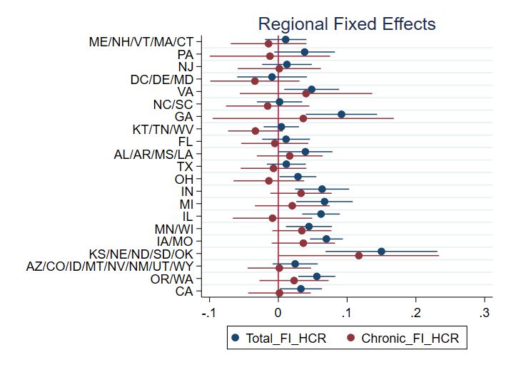
Unpacking the patterns in Figure 3 by household heads’ race, gender and
educational attainment, we see in Table 5 and Figure 4 that both the prevalence
and persistence of food insecurity are markedly higher among households headed by
women, those without a high school degree, the physically disabled, and SNAP recip-
ients. Households whose head lost his or her job have especially high food insecurity
persistence rates. Households whose head became unmarried through separation,
divorce or death have especially low food insecurity persistence rates.
Figure 4 depicts the groupwise dynamics of food insecurity prevalence, divided
among those who newly became food insecure in a PSID survey year (top panel, a)
and those who remained food insecure, having been so in the prior survey wave as well
(bottom panel, b). These graphics reflect the combination of sub-group population
sizes as well as the group-specific transitions reflected in Table 5. Both panels clearly
show vulnerable subgroups’ disproportionately high rates of entry and persistence.
22Note: Sample includes households with non-missing PFS from 2003 to 2017.
“Still food insecure” and “Newly food insecure” refer to households that were
or were not food insecure in the preceding survey wave, respectively. “Previous
status unknown” refers to households whose PFS in the preceding wave is miss-
ing. The prevalence reported at the top of each bar matches the official HFSM
by construction
Figure 3: Change in Food Security Status
23Note: Sample includes households with non-missing PFS from 2003 to 2017. ”Still
food insecure” and ”Newly food insecure” refer to food insecure households that
were and were not food insecure in the preceding survey wave, respectively. “HS”
indicates the head has no education beyond high school. “Col” indicates that
the head has at least some college education. “Color” indicates the head is a
person of color. Percentages in parentheses report each category’s share of the
total population.
Figure 4: Change in Food Security Status by Group
24For example, over this period, female-headed households accounted for 22.4% of the
population but 40% of the newly food insecure and 60% of persistently food insecure
households. The ratio of newly food insecure households increased by 70% during
the Great Recession between 2007 to 2009 (3.6% to 6.1%) where 30% of the increase
consisted of households whose head is female without a college education. That same
sub-group accounted for 54% of the reduction in newly food insecure households
in the post-Great Recession recovery. By contrast, the most vulnerable sub-group
- households headed by non-White women with no high school degree - exhibited
a relatively stable entry rate before and after the recession and by far the highest
persistence rate. Households headed by white women with no more than a high
school degree accounted for the largest share (27%) of still food insecure households
immediately after the Great Recession (2009-2011).
3.3 Household-level Dynamics: Permanent Approach
Turning to the permanent approach to the study of food insecurity dynamics,
Table 6 columns (1) to (4) report the estimated chronic component (CFI) of total
food insecurity (TFI) measures from the headcount ratio (HCR), following equation
(4) and (5) with α = 0. Columns (5) to (8) then show the distribution of households
among those who are chronically and persistently food insecure (column 5), chroni-
cally food insecure but transiently food secure some periods (column 6), those who
are occasionally food insecure but on average food secure (column 7), and those never
food insecure (column 8)19 .
Overall, nearly 70% of households never experienced food insecurity over the 17
years we study. Persistent food security is thus the dominant state in the population.
But among the 30% who are food insecure, 74% of the food insecurity households
experience is chronic, meaning expected in every period. Sub-group analyses again
show households whose head is female or non-White or have not completed high
school have sharply higher rates of TFI. Perhaps most strikingly, CFI falls in the
19. We test for nonstationarity in the PFS series using the Fisher-type panel data unit-root test
and an augmented Dickey–Fuller (ADF) test for each household (Choi 2001). Assuming no trend
in the data generating process, we reject the null hypothesis that all the panels have unit roots,
implying that at least one panel is stationary. This a weak test but provides some assurance that
the permanent approach is not compromised by nonstationarity in the PFS series.
25Table 6: Chronic Food Insecurity Status from the Permanent Approach
(1) (2) (3) (4) (5) (6) (7) (8)
N TFI CFI TFI-CFI (CFI/TFI) Chronic Transient Never food insecure
Persistent Not persistent
Total 22,324 0.124 0.092 0.032 0.744 0.026 0.066 0.210 0.698
Gender
Male 17,291 0.076 0.044 0.032 0.577 0.010 0.034 0.191 0.765
Female 5,033 0.288 0.259 0.030 0.896 0.083 0.176 0.276 0.466
Race
White 14,937 0.086 0.052 0.034 0.605 0.011 0.041 0.198 0.750
Non-White 7,387 0.345 0.327 0.018 0.947 0.113 0.213 0.283 0.390
Region
Northeast 1,525 0.046 0.034 0.013 0.727 0.004 0.029 0.090 0.876
Mid-Atlantic 3,022 0.110 0.079 0.031 0.722 0.014 0.066 0.205 0.716
26
South 7,942 0.147 0.120 0.027 0.819 0.042 0.078 0.203 0.677
Midwest 5,401 0.146 0.104 0.042 0.709 0.036 0.068 0.248 0.649
West 4,316 0.115 0.082 0.033 0.711 0.015 0.067 0.226 0.693
Metropolitan area
Metropolitan 15,532 0.115 0.084 0.031 0.727 0.026 0.058 0.197 0.719
Non-metropolitan 6,719 0.145 0.112 0.033 0.774 0.028 0.085 0.242 0.646
Education
Less than HS 3,307 0.355 0.318 0.036 0.898 0.114 0.205 0.338 0.344
High school 7,259 0.148 0.105 0.043 0.708 0.023 0.082 0.282 0.613
Some college 5,472 0.098 0.065 0.033 0.666 0.020 0.045 0.199 0.736
College 6,286 0.042 0.023 0.020 0.535 0.003 0.019 0.114 0.864
Note: Sample include households with non-missing PFS for 5 or more years from 2001 to 2017. The food insecurity measure is the headcount ratio (HCR) using the PFS following the
method from Jalan and Ravallion (2000). Metropolitan area include the counties in metropolitan area with 250,000 or more population. States excluding Alaska and Hawaii belong to
one of the five regions as described in Table A3. AK, HA and other U.S. territories are excluded in regional categories The last four columns describe the distribution of households
status which add up to one.You can also read