Fundamentals of Radio Astronomy - Cornelia C. Lang, University of Iowa
←
→
Page content transcription
If your browser does not render page correctly, please read the page content below
ITN 215212: Black Hole Universe
          1st School on Multiwavelength Astronomy     1
                   Paris: 29 June – 10 July

         Fundamentals of Radio
              Astronomy

     Cornelia C. Lang, University of Iowa

          Many slides taken from NRAO
        Synthesis Imaging Summer School

   Lectures by Perley, McKinnon, Myers, Carilli:
See: http://www.aoc.nrao.edu/events/synthesis/2008/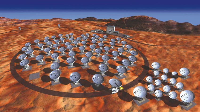
Fundamentals of Radio Astronomy                                           2

• Radio Emission: what can we learn?
  –   Thermal and non-thermal continuum emission, spectral line radiation
  –   The radio spectrum (“lo, mid and high”)
  –   Interferometers and single dish instruments
  –   Science results – what can you do with radio?
• Antenna Theory & Receivers
  – Basic description, power patterns and directionality
  – Heterodyne receivers (centimeter-wave)
• Polarization
  – Basic concepts and examples; relation to Stokes parameters
• Interferometry Basics
  – Getting better resolution
  – Signal multiplication, correlation function and making an image
  – Sensitivity of an interferometer
Fundamentals of Radio Astronomy                              3

• Equations that you should remember:
- Resolution of an interferometer = 1.02 λ/D where
D = baseline length (i.e., 25 km for the VLA)

- Field of view of an interferometer = primary beam =
1.02 λ/D where D = dish diameter (i.e., 25 m for the VLA)
- Polarization in terms of Stokes parameters =

-   Visibility function and its relation to sky brightness (FT)

-   Sensitivity equation (radiometer equation)
4
       Radio Emission Mechanisms

• Synchrotron radiation - continuum
    • Energetic charged particles accelerating along
      magnetic field lines (non-thermal)
                                            • What can we
                                                learn?
                                         • particle energy

                                         • strength of
                                         magnetic field

                                         • polarization

                                         • orientation of
                                         magnetic field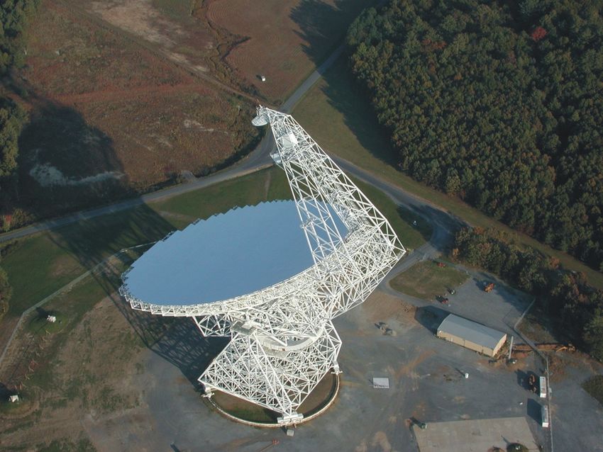
5
              Radio Emission Mechanisms

• Thermal emission - continuum
       • Blackbody radiation for objects with T~3-30 K
       • Brehmsstralung “free-free” radiation: charged particles
         interacting in a plasma at T; e- accelerated by ion

Hα image                             • What can we learn?

                                      • mass of ionized gas
                                      • optical depth
                                      • density of electrons in plasma
                                      • rate of ionizing photons

           Courtesy of Dana Balser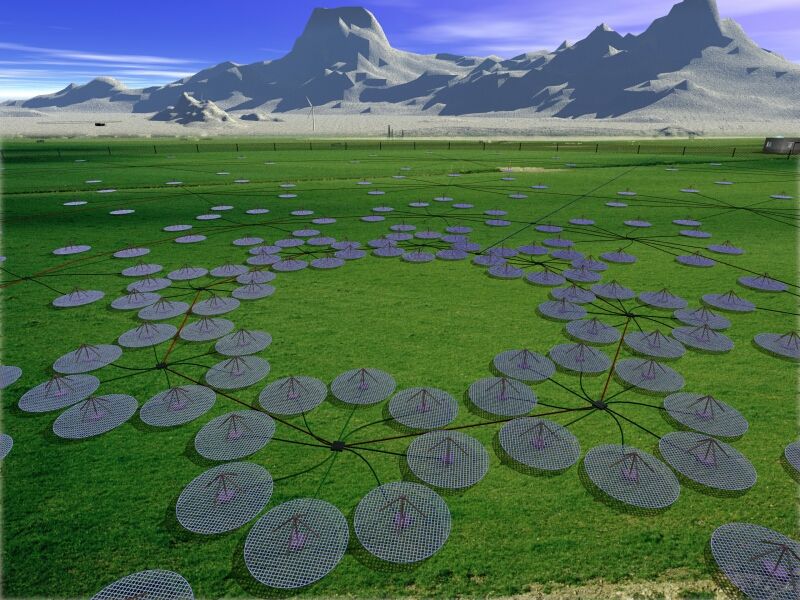
6
Radio Emission Mechanisms
• What we measure from radio continuum
• Radio flux or flux density at different frequencies
• Spectral index α, where Sν ~ να
Spectral index across a SNR
Flux or Flux Density
thermal α = -0.1
From T. Delaney
Frequency 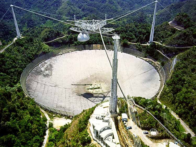
7
      Radio Emission Mechanisms

• Spectral line emission
 - Discrete transitions in atoms and molecules

             Atomic Hydrogen
            “spin-flip” transition
                   21 cm

                                            Molecular Lines
            Recombination Lines          CO, CS, H20, SiO, etc.!
            outer transitions of H
            H166α, H92α, H41α • What can we learn?
           (1.4, 8.3 GHz, 98 GHz)
                                   • gas physical conditions (n, T)
                                   • kinematics (Doppler Effect)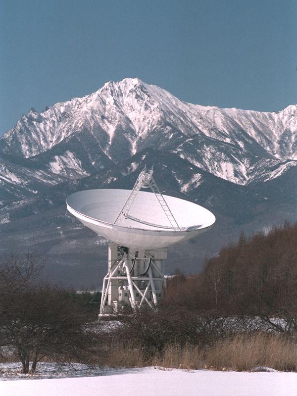
A wide variety of single dishes!                            8

                                        Nobeyama,
              Parkes, AUS                 Japan

                            GBT, USA
Millimeter                                          Low-Frequency
> 15 GHz                                              < 1.4 GHz
< 10 mm                                                 >1m

      IRAM                     Centimeter             Arecibo, USA
      Spain                 1.4 MHz - 15 GHz
                              20 cm – 1 cm

LMT, Mexico   CSO, Hawaii              Lovell, UK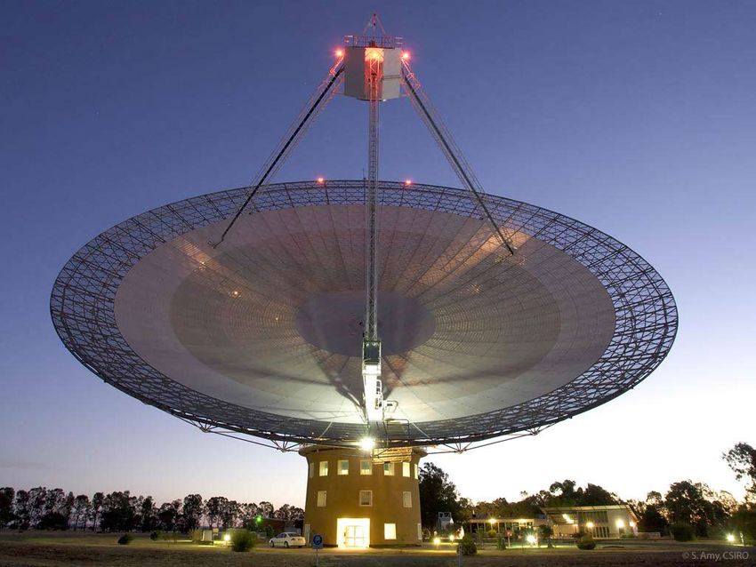
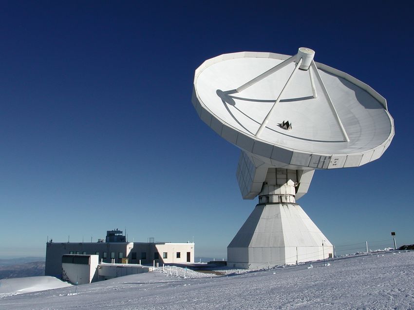
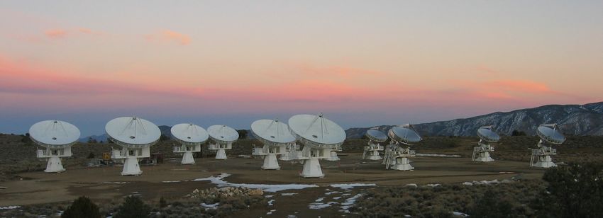
A wide variety of interferometers!                               9

                    ATA
                  CA, USA              VLA/EVLA
                                       NM, USA
                     ATCA, Australia
   Millimeter                                           Low-Frequency
   > 15 GHz                                               < 1.4 GHz
   < 10 mm                                                  >1m

                                  Centimeter
                               1.4 MHz - 15 GHz
                                 20 cm – 1 cm

                ALMA, Chile                                    GMRT, India
   PdB,                                           LOWFAR, NL
  France
CARMA,
CA, USA

                         SMA, Hawaii, USA                      LWA, NM, USA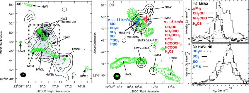
Resolution of a radio telescope                       10

• Resolution of a single dish radio telescope: 1.02 λ/D where
D = diameter of telescope; therefore, VLA @20 cm: 30’ resol.

• Resolution of an interferometer: 1.02 λ/D where D longest
baseline: VLA @ 20 cm with 30 km baseline = few arcseconds

• Primary beam (or “field of view”) for int. = single dish resol.

                                        For ALMA, baselines of
                                            Up to 15 km !!

                                        Wavelengths: < 1 mm

                                           Resolutions: < 1”!
11
Tour of the Galaxy: Interstellar
• Low Mass Star Formation
- obscured regions of the Galaxy with high resolution
- collimated outflows powered by protostar – 10000s AU
Chandler & Richer 2001
Zapata et al. 2005
VLA 7mm spectral line (SiO) – 0.5” SMA 1mm spectral line (CO 2-1) – 1”12
Tour of the Galaxy: Interstellar
• Probing massive stars in formation
- tend to be forming in clusters; confusion! go to high frequencies (sub-mm)
- “hot molecular cores” (100-300K) around protostars; complex chemistry
Ceph A-East d=725 pc; black=SMA 875 µm; green=VLA 3 cm; lines=sub-mm species
Spatial resolutions of13
Tour of the Galaxy: Interstellar
• Star Death: Pulsar Wind Nebulae
G54 VLA B-field
Chandra X-ray Image Chandra X-ray Image
2.5’ @
2.7’ @ d=2 kpc
d=5 kpc ~ 1.4 pc
~ 3. 8 pc
G54 VLA 6 cm
G54.1+0.3 Crab
Lang et al., submitted.
radio studies: particle energies, polarization, magnetic field orientation
VLA/VLBA pulsar proper motion can be combined with spin-axis orientation (X-ray)
Pulsar timing and discovery done with single dish radio telescopes – Parkes, GBT14
Tour of the Galaxy: Stellar Sources
• Stars: Very low mass and brown dwarfs
- some M+L type dwarfs, brown dwarfs show quiescent and flaring non-
thermal emission (Berger et al. 2001-7; Hallinan et al. (2006,2008)15
Tour of the Galaxy: Exotic
• LS I+61 303 : A pulsar comet around a hot star?
- well known radio, X-, γ ray, source
----------
Orbital 10 AU
- high mass X-ray binary with Phase
12 solar mass Be star and NS
- radio emission models:
(a) accretion-powered jet or
(b) rotation powered pulsar
-VLBA data support pulsar model
in which particles are shock-
accelerated in their interaction with VLBA 3.6 cm; 3 days apart!
Note shift of centroid around orbit
the Be star wind/disk environment
Astrometry is good to rms = 0.2 AU
(Dhawan, Mioduszewski & Rupen 2006)16
Tour of the Galaxy: Exotic
• LS I+61 303 : A pulsar comet around a hot star?
Orbit greatly exaggerated
VLBA emission vs. orbital phase
Be star (with wind/disk)
Dhawan, Mioduszewski & Rupen (2006)Center of our Galaxy VLA 20cm 17
VLA 1.3cm
VLA 3.6cm
SgrA* - 4 milliion Mo
black hole source
Credits: Lang, Morris, Roberts, Yusef-Zadeh, Goss, Zhao18
Tour of the Galaxy: The Galactic Center
• Magnetic Field: Pervasive vs. Local?
VLA 3.6 & 6 cm
VLA 90 cm
polarization
B-field
Nord et al. 2004
Lang & Anantharamaiah, in prep.Radio Spectral Lines: Cold Gas 19
20
    Jet Energy via Radio Bubbles in Hot Cluster Gas

     1.4 GHz VLA contours over Chandra X-ray image (left) and optical (right)
6 X 1061 ergs ~ 3 X 10⁷ solar masses X c2 (McNamara et al. 2005, Nature, 433, 45)
21 Resolution and Surface-brightness Sensitivity
Superluminal Motion in
                               22
    Compact Jets

 First major VLBI discovery:
    apparent superluminal
  motion, implying compact
      jets moving highly
        relativisitically.
Resolving the circumnuclear disk in NGC 4258
23
and directly measuring the black-hole mass
NGC 4258
NGC 4258
r
H20 masers: get speed, period, positional accuracy (10 microarcseconds!)
directly measures SMBH masses, proper motions, acceleration, encl. density24
Types of Antennas
• Wire antennas
Yagi
– Dipole
– Yagi
– Helix Helix
– Small arrays of the above
• Reflector antennas
• Hybrid antennas
– Wire reflectors
– Reflectors with dipole
feedsAntennas – the Single Dish 25 • The simplest radio telescope (other than elemental devices such as a dipole or horn) is a parabolic reflector – a ‘single dish’ with associated feed(s). • Four important characteristics of an antenna: – They have a directional gain. – They have an angular resolution given by: θ ~ λ/D. – They have ‘sidelobes’ – finite response at large angles. – Their angular response contains no sharp edges. • A basic understanding of the origin of these characteristics will aid in understanding the functioning of an interferometer.
26
                       Basic Antenna Formulas
Effective collecting
area A(ν,θ,φ) m2

On-axis response A0 = ηA
η = aperture efficiency

Normalized pattern
(primary beam)
A(ν,θ,φ) = A(ν,θ,φ)/A0

Beam solid angle
ΩA= ∫∫ A(ν,θ,φ) dΩ
   all sky

A0 ΩA = λ2
λ = wavelength, ν = frequency
The Standard Parabolic Antenna Response 27 - “illumination” helps to determine this response - This response important because you want to “clean” out emission from sidelobes and restore into your main beam (little different for an interferometer)
Reflector Optics: Examples                   28

Prime focus                            Cassegrain focus
  (GMRT)                                 (AT)

Offset Cassegrain                      Naysmith
  (VLA)                                (OVRO)

Beam Waveguide                               Dual Offset
  (NRO)                                    (GBT)
29
      Feed Systems

      EVLA           GBT

ATA
Antenna Performance: Aperture
30
Efficiency
On axis response: A0 = ηA
Efficiency: η = ηsf × ηbl × ηs × ηt × ηmisc
ηsf = Reflector surface efficiency rms error σ
Due to imperfections in reflector surface
ηsf = exp( (4πσ/λ)2) e.g., σ = λ/16 , ηsf = 0.5
ηbl = Blockage efficiency
Caused by subreflector and its support structure
ηs = Feed spillover efficiency
Fraction of power radiated by feed intercepted by subreflector
ηt = Feed illumination efficiency
Outer parts of reflector illuminated at lower level than inner part
ηmisc= Reflector diffraction, feed position phase errors, feed match and lossVLA @ 4.8 GHz (C-band) Interferometer Block Diagram 31
Antenna
Front End
IF
Key
Amplifier
Mixer Back End
X Correlator
Correlator32
The Polarization Ellipse
• From Maxwell’s equations E•B=0 (E and B perpendicular)
– By convention, we consider the time behavior of the E-field in
a fixed perpendicular plane, from the point of view of the
receiver.
• For a monochromatic wave of frequency ν, we write
E x = Ax cos(2πυ t + φ x )
E y = Ay cos(2πυ t + φ y )
– These two equations describe an ellipse in the (x-y) plane.
• The ellipse is described fully by three parameters:
– A ,€
X A , and the phase difference, δ = φ -φ .
Y Y X
• The wave is elliptically polarized. If the E-vector is:
– Rotating clockwise, the wave is ‘Left Elliptically Polarized’,
– Rotating counterclockwise, it is ‘Right Elliptically Polarized’.33
Stokes parameters
• Spherical coordinates: radius I, axes Q, U, V
– I = EX2 + EY2 = ER2 + EL2
– Q = I cos 2χ cos 2ψ = EX2 - EY2 = 2 ER EL cos δRL
– U = I cos 2χ sin 2ψ = 2 EX EY cos δXY = 2 ER EL sin δRL
– V = I sin 2χ = 2 EX EY sin δXY = ER2 - EL2
• Only 3 independent parameters:
– wave polarization confined to surface of Poincare sphere
– I2 = Q2 + U2 + V2
• Stokes parameters I,Q,U,V
– defined by George Stokes (1852)
– form complete description of wave polarization
– NOTE: above true for 100% polarized monochromatic wave!34
Linear Polarization
• Linearly Polarized Radiation: V = 0
– Linearly polarized flux:
– Q and U define the linear polarization position angle:
– Signs of Q and U:
Q>0
U>0 U35
Simple Examples
• If V = 0, the wave is linearly polarized. Then,
– If U = 0, and Q positive, then the wave is vertically polarized,
Ψ=0°
If U = 0, and Q negative, the wave is horizontally polarized,
Ψ=90°
– If Q = 0, and U positive, the wave is polarized at Ψ = 45°
– If Q = 0, and U negative, the wave is polarized at Ψ = -45°.Illustrative Example: Non-thermal Emission from Jupiter 36
• Apr 1999 VLA 5 GHz data
• D-config resolution is 14”
• Jupiter emits thermal
radiation from atmosphere,
plus polarized synchrotron
radiation from particles in its
magnetic field
• Shown is the I image
(intensity) with polarization
vectors rotated by 90° (to
show B-vectors) and
polarized intensity (blue
contours)
• The polarization vectors
trace Jupiter’s dipole
• Polarized intensity linked to
the Io plasma torus37
Example: Radio Galaxy 3C31
• VLA @ 8.4 GHz
• E-vectors
– along core of jet
– radial to jet at edge
• Laing (1996)
3 kpc38
Example: Radio Galaxy Cygnus A
• VLA @ 8.5 GHz B-vectors Perley & Carilli (1996)
10 kpc39
Getting Better Resolution: Interferometry
• The 25-meter aperture of a VLA antenna provides insufficient
resolution for modern astronomy.
– 30 arcminutes at 1.4 GHz, when we want 1 arcsecond or better!
• The trivial solution of building a bigger telescope is not
practical. 1 arcsecond resolution at λ = 20 cm requires a 40
kilometer aperture.
– The world’s largest fully steerable antenna (operated by the NRAO
at Green Bank, WV) has an aperture of only 100 meters ⇒ 4 times
better resolution than a VLA antenna.
• As this is not practical, we must consider a means of
synthesizing the equivalent aperture, through combinations of
elements.
• This method, termed ‘aperture synthesis’, was developed in the
1950s in England and Australia. Martin Ryle (University of
Cambridge) earned a Nobel Prize for his contributions.40
Establishing Some Basics
• Consider radiation from direction s from a small elemental solid
angle, dΩ, at frequency ν within a frequency slice, dν.
• For sufficiently small dν, the electric field properties (amplitude,
phase) are stationary over timescales of interest (seconds), and
we can write the field as
• The purpose of an antenna and its electronics is to convert this
E-field to a voltage, V(t) – proportional to the amplitude of the
electric field, and which preserves the phase of the E-field –
which can be conveyed from the collection point to some other
place for processing.
• We ignore the gain of the electronics and the collecting area of
the antennas – these are calibratable items (‘details’).
• The coherence characteristics can be analyzed through
consideration of the dependencies of the product of the voltages
from the two antennas.The Stationary, Quasi-Monochromatic Interferometer 41
• Consider radiation from a small solid angle dΩ, from direction s, at
frequency ν, within dν:
s s
Geometric The path lengths
Time Delay from antenna
to correlator are
assumed equal.
b An antenna
X
multiply
average42
Examples of the Signal Multiplications
The two input voltages are shown in red and blue, their product is in black.
The desired coherence is the average of the black trace.
In Phase: ωτg = 2πn
RC = A 2 /2
Quadrature Phase:
ωτg = (2n+1)π/2
Anti-Phase:
ωτg = (2n+1)π43
Signal Multiplication, cont.
• The averaged product RC is dependent on the source power, A2 and
geometric delay, τg:
– RC is thus dependent only on the source strength, location, and baseline
geometry.
• RC is not a a function of:
– The time of the observation (provided the source itself is not variable!)
– The location of the baseline, provided the emission is in the far-field.
• The strength of the product is also dependent on the antenna areas
and electronic gains – but these factors can be calibrated for.
• We identify the product A2 with the specific intensity (or brightness) Iν
of the source within the solid angle dΩ and frequency slice dν.44
The Response from an Extended Source
• The response from an extended source is obtained by summing
the responses for each antenna over the sky, multiplying, and
averaging:
• The expectation, and integrals can be interchanged, and
providing the emission is spatially incoherent, we get
• This expression links what we want – the source brightness on
the sky, Iν(s), – to something we can measure - RC, the
interferometer response.A Schematic Illustration of Correlation 45
• The correlator can be thought of ‘casting’ a sinusoidal coherence
pattern, of angular scale λ/b radians, onto the sky.
• The correlator multiplies the source brightness by this coherence
pattern, and integrates (sums) the result over the sky.
• Orientation set by baseline
geometry.
• Fringe separation set by
(projected) baseline length and λ/b rad.
wavelength.
• Long baseline gives close- Source
packed fringes brightness
• Short baseline gives widely-
separated fringes
• Physical location of baseline
unimportant, provided source is + + + Fringe Sign
in the far field.46
Odd and Even Functions
• But the measured quantity, Rc, is insufficient – it is only
sensitive to the ‘even’ part of the brightness, IE(s).
• Any real function, I, can be expressed as the sum of two
real functions which have specific symmetries:
An even part: IE(x,y) = (I(x,y) + I(-x,-y))/2 = IE(-x,-y)
An odd part: IO(x,y) = (I(x,y) – I(-x,-y))/2 = -IO(-x,-y)
IE IO
I
= +Recovering the ‘Odd’ Part: The SIN Correlator 47 The integration of the cosine response, Rc, over the source brightness is sensitive to only the even part of the brightness: since the integral of an odd function (IO) with an even function (cos x) is zero. To recover the ‘odd’ part of the intensity, IO, we need an ‘odd’ coherence pattern. Let us replace the ‘cos’ with ‘sin’ in the integral: since the integral of an even times an odd function is zero. To obtain this necessary component, we must make a ‘sine’ pattern.
48
                     Making a SIN Correlator

•   We generate the ‘sine’ pattern by inserting a 90 degree phase shift
    in one of the signal paths.
                            s                      s

                             b                     An antenna

                                X   90o
       multiply

       average
49
Define the Complex Visibility
We now DEFINE a complex function, V, to be the complex sum of the
two independent correlator outputs:
where
This gives us a beautiful and useful relationship between the source
brightness, and the response of an interferometer:
Although it may not be obvious (yet), this expression can be inverted to
recover I(s) from V(b).50
Making Images
We have shown that under certain (and attainable)
assumptions about electronic linearity and narrow
bandwidth, a complex interferometer measures the
visibility, or complex coherence:
(u,v) are the projected baseline coordinates,
measured in wavelengths, on a plane oriented facing the
phase center, and
(l,m) are the sines of the angles between the phase
center and the emission, in the EW and NS directions,
respectively.51
Making Images
This is a Fourier transform relation, and it can be in
general be solved, to give:
This relationship presumes knowledge of V(u,v) for all
values of u and v. In fact, we have a finite number, N,
measures of the visibility, so to obtain an image, the
integrals are replaced with a sum:
If we have Nv visibilities, and Nm cells in the image, we have
~NvNm calculations to perform – a number that can exceed 1012!VLA @ 4.8 GHz (C-band) Interferometer Block Diagram 52
Antenna
Front End
IF
Key
Amplifier
Mixer Back End
X Correlator
CorrelatorImportance of Antennas for Interferometers 53 • Antenna amplitude pattern causes amplitude to vary across the source. • Antenna phase pattern causes phase to vary across the source. • Polarization properties of the antenna modify the apparent polarization of the source. • Antenna pointing errors can cause time varying amplitude and phase errors. • Variation in noise pickup from the ground can cause time variable amplitude errors. • Deformations of the antenna surface can cause amplitude and phase errors, especially at short wavelengths.
Some radio astronomy definitions 54
Interferometric Radiometer Equation                55

• Tsys = wave noise for photons (RJ): rms ∝ total power
• Aeff,kB = Johnson-Nyquist noise + antenna temp
definition
• tΔν = # independent measurements of TA/Tsys per pair
of antennas
• NA = # indep. meas. for array, or can be folded into
Aeff
56
                    Summary

• Radio Interferometry: a powerful tool
  – Physical insight into many different processes
  – Spatial scales comparable or better than at other
    wavelengths: multi-wavelength approach

• A great time for students & interferometry!
  – Amazing science opportunities with new tools
             ATA             EVLA     LOFAR
    CARMA

                     ALMA
                                              LWA
You can also read