Gene Expression Programming and Machine Learning Methods for Bushre Susceptibility Mapping in New South Wales, Australia
←
→
Page content transcription
If your browser does not render page correctly, please read the page content below
Gene Expression Programming and Machine Learning Methods for
Bushfire Susceptibility Mapping in New South Wales, Australia
Maryamsadat Hosseini ( maryamsadat.hosseini@unsw.edu.au )
University of New South Wales https://orcid.org/0000-0002-2858-9705
Samsung Lim
University of New South Wales
Research Article
Keywords: Gene expression programming, Bushfire, Susceptibility map, Machine learning.
Posted Date: September 28th, 2021
DOI: https://doi.org/10.21203/rs.3.rs-828738/v1
License: This work is licensed under a Creative Commons Attribution 4.0 International License. Read Full License
Page 1/14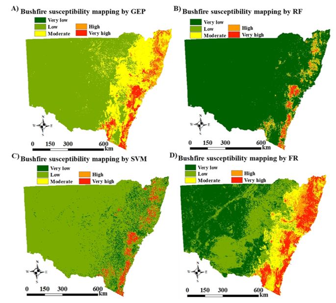
Abstract
Australia is one of the most bushfire-prone countries. Prediction and management of bushfires in bushfire-susceptible areas can reduce the
negative impacts of bushfires. The generation of bushfire susceptibility maps can help improve the prediction of bushfires. The main aim of this
study was to use single gene expression programming (GEP) and ensemble of GEP with well-known statistical methods to generate bushfire
susceptibility maps for New South Wales, Australia as a case study. We used eight methods for bushfire susceptibility mapping: GEP, random
forest (RF), support vector machine (SVM), frequency ratio (FR), ensemble techniques of GEP and FR (GEPFR), RF and FR (RFFR), SVM and FR
(SVMFR), and LR and FR (LRFR). Areas under the curve (AUCs) of the receiver operating characteristic were used to evaluate the proposed
methods. GEPFR exhibited the best performance for bushfire susceptibility mapping based on the AUC (0.890), while RFFR had the highest
accuracy (94.70%) among the proposed methods. GEPFR is an ensemble method that uses features from the evolutionary algorithm and the
statistical FR method, which results in a better AUC for the bushfire susceptibility maps. The ensemble methods had better performances than
those of the single methods.

1. Introduction
Australia has been suffering more from bushfires than other types of natural disasters in recent years due to climate changes which have
increased the temperature and decreased rainfalls (Yu et al. 2020). Bushfires can be harmful to the human health and cause devastating
impacts on the environment and economy (Zhang et al. 2016). For example, 173 people were killed and 1.1 million acres of area were burned
during Black Saturday bushfires in Australia in 2009 (Ma et al. 2020). Later, 248 buildings across the New South Wales (NSW) were destroyed by
bushfires in 2013 (Ma et al. 2020). The most catastrophic bushfire season occurred in the summer of 2019/2020, which devastated fire-fighters,
humans, and animals (Milton and White 2020). The frequency and severity of the bushfires are expected to increase in the future as a result of
climate changes (Milton and White 2020). It is important to model bushfires and mitigate the negative impacts of bushfires on humans and
environment. It is also important to determine areas with a high possibility of bushfire occurrence to achieve a better natural hazard
management (Tehrany et al. 2021). Various algorithms and methods have been applied to bushfire susceptibility mapping (Tehrany et al. 2021),
including statistical methods, artificial intelligence and machine learning (ML) techniques, ensemble techniques, and evolutionary algorithms.

Statistical methods have been used to generate bushfire susceptibility maps in different studies, such as frequency ratio (FR), evidential belief
function (EBF), and weight of evidence (WOE) (Pourghasemi 2016; Hong et al. 2017, 2019; Jaafari et al. 2017). FR uses an understandable
procedure and simplifies the problem and outcome, which enables to analyze large datasets in software such as ArcGIS (Pradhan et al. 2007).
Statistical methods can be used in the ArcGIS environment, which enables to generate spatial patterns of bushfire prediction maps (Nami et al.
2018).

Bushfire susceptibility mapping in a case study on Minudasht forests in Iran showed that Shannon’s entropy (SE) and FR are two promising
methods for the prediction of bushfires with areas under the curve (AUCs) of 83.16% and 79.85%, respectively (Pourtaghi et al. 2015). EBF is
also an appropriate statistical method for the prediction of bushfires, with an AUC of 81.03% in the Hyrcanian ecoregion in Iran (Nami et al.
2018). Another study also showed that logistic regression (LR) and FR had bushfire prediction rates of 88.3% and 85.3% in Thimphu and Paro
districts in western Bhutan (Dorji and Ongsomwang 2017), respectively.

A study in the Yihuang area, China, showed that the methods such as linear discriminant analysis and quadratic discriminant analysis (LDA and
QDA), FR, and WOE were useful for the prediction of bushfires. WOE had the highest AUC (82.20%), followed by FR (80.9%), QDA (78.3%), and
LDA (78.0%) (Hong et al. 2017).

The advancement of remote-sensing technologies has improved the bushfire management and monitoring (Jain et al. 2020). The bushfire
prediction by data-driven methods has recently been used owing to the improvement in data quality (e.g., weather data) (Jain et al. 2020). The
advancement in data quality has also helped scientists to use different ML techniques for bushfire susceptibility mapping (Jain et al. 2020). ML
techniques can predict bushfires using input data, regardless of the expert’s knowledge. ML techniques are trained by a portion of the data and
find the most fitted model that can be used for the generation of spatial maps for the bushfire prediction in the entire bushfire-prone area
(Leuenberger et al. 2018; Tonini et al. 2020).

Recent studies have shown that new artificial intelligence methods generate more accurate results than conventional statistical techniques
(Hoang and Tien Bui 2018). Different ML methods such as random forest (RF), artificial neural network (ANN), decision tree (DT), support vector
machine (SVM), and genetic algorithms (GAs) have been applied to bushfire prediction (Jain et al. 2020). The application of multiple ML
methods, including RF, ANN, multi-layer perceptron (MLP), Dmine regression (DR), least-angle regression, radial basis function (RBF), self-
organized map, SVM, DT, and LR showed that RF had the highest AUC (88.0%) for the prediction of bushfires in Mazandaran province, Iran
(Gholamnia et al. 2020). Similarly, RF provided promising results during different seasons in the Liguria region of Italy (Tonini et al. 2020). RF
exhibited better results than those of SVM, ANN, LR, and Probit regression (Cao et al. 2017; Ghorbanzadeh et al. 2019).

                                                                   Page 2/14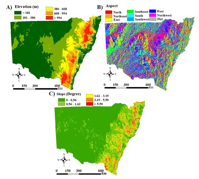
Unlike deterministic methods, RF does not require prior knowledge of the bushfires, yet achieves a similar accuracy as those of deterministic
methods (Leuenberger et al. 2018). Other ML methods such as Bayes network (BN), DT, naive Bayes (NB), and multi-variate logistic regression
(MLR) have been applied to the bushfire prediction in Pu Mat National Park, Vietnam (Pham et al. 2020). The BN had an AUC of 96.0%, followed
by DT (94.0%), NB (93.9%), and MLR (93.7%) (Pham et al. 2020). Kernel logistic regression and SVM were also used to generate bushfire
susceptibility maps in Cat Ba National Park, Vietnam, where the kernel logistic regression had the highest AUC of 92.2% for the prediction of
bushfires (Bui et al. 2016).

Ensembles of ML methods also showed promising outcomes for bushfire susceptibility mapping. The ensemble of different techniques,
including ANFIS, GA, and simulated annealing (SA), had the highest AUC of 90.3% for the bushfire prediction (Razavi-Termeh et al. 2020).
Razavi-Termeh et al. (2020) also reported that an ensemble of RBF and an imperialist competitive algorithm had an AUC of 87.8%. A
combination of WOE and a knowledge-based analytical hierarchy process was more accurate than the use of WOE alone and LR in Huichang
County, China (Hong et al. 2019).

Gene expression programming (GEP) which is a branch of artificial intelligence approaches proposed by Ferreira (2001), can find the explicit
function between the response variables and conditioning factors automatically without considering assumptions about the problem’s function
form (Ferreira 2001; Emamgolizadeh et al. 2015; Hoang and Tien Bui 2018). GEP determines the relationships between dependent variables and
conditioning factors that can be nonlinear (Hosseini and Lim 2021). GEP is a useful tool for natural disaster prediction such as landslide
prediction (Zakaria et al. 2010; Kayadelen 2011; Mousavi et al. 2012; Hoang and Tien Bui 2018; Hosseini and Lim 2021).

The main purpose of this research is to investigate the application of GEP for generating bushfire probability maps. GEP is a relatively new
approach based on an evolutionary algorithm. Therefore, our models generated by GEP are expected to provide some important insights to
bushfire susceptibility mapping. To implement GEP and measure its capability to produce bushfire susceptibility maps over NSW which is one of
the most bushfire-prone states in Australia, we proposed four ensemble methods: GEP and FR (GEPFR), RF and FR (RFFR), SVM and FR
(SVMFR), LR and FR (LRFR), and four baseline methods: GEP, RF, SVM, and FR for the comparison with the ensemble methods. We compared
the results of single and ensemble methods to identify the best method for the prediction of bushfires in our case study area.

2. Methods
2.1. Study area
The study area is NSW, in the eastern part of Australia, located at latitudes of 28˚ 15' S to 37˚ 30' S and longitudes of 141˚ E to 153˚ 30' E
(Fig. 1). NSW has an area of 801,150 km2 and its elevation ranges from − 7 m to 2,175 m. Queensland is located to the north of NSW, while
South Australia is located on the west side of NSW. NSW borders Victoria to the south. From the east, NSW has coast borders with Coral and
Tasman Seas. Plant covers in NSW mainly include grassland, shrubland, savannas, and forests.

2.2. Data preparation
2.2.1. Bushfire inventory map
Data collection is an important step before the generation of bushfire susceptibility maps (Eskandari et al. 2020). The generation of an inventory
map is the first step in establishing a GIS database (Hoang and Tien Bui 2018). The bushfire inventory map in NSW was generated from the
MODIS fire data (MODIS 500-m MCD 64 Monthly). These data were collected for the period of the fire season in Australia (November to
February) between 2010 and 2020 (Fig. 1). In this study, 70% of the inventory map was randomly allocated to the training set, while the
remaining 30% was used for the testing set (Eskandari et al. 2020).

2.2.2. Conditioning factors
Bushfire is a complex phenomenon. Numerous factors can contribute to bushfire occurrence. As a result, the selection of conditioning factors is
an important step for the generation of bushfire susceptibility maps (Eskandari et al. 2020). In this study, we selected topography, climate, fuel
loads, and human-made factors as conditioning factors based on the availability of data (Jaafari et al. 2017, 2019; You et al. 2017; Sachdeva et
al. 2018; Hong et al. 2019; Zhang et al. 2019; Eskandari et al. 2020; Tonini et al. 2020).

Slope, aspect, and digital elevation model (DEM) were used as topographical factors in this study. The DEM (ASTER 30-m GDEM) is illustrated in
Fig. 2A. DEM data were collected from the United States Geological Survey (USGS) website (USGS 2021). Elevation is another important factor
in bushfire occurrence (Gigović et al. 2019). The aspect and slope were derived from the DEM (Figs. 2B and 2C, respectively). Slope is the land
gradient, represented in percentages or angles, which has a significant impact on the bushfire behavior (Gigović et al. 2019). The burn speed is
higher on a steep slope. The slope can impact the direction of the bushfire (Gigović et al. 2019). Aspect is the direction of the slope and
influences the slope in connection with insolation and exposure to wind (Gigović et al. 2019).

                                                                     Page 3/14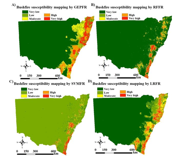
The climatic factors used in this study are annual mean precipitation and annual maximum temperature. These data were collected from the
Bureau of Meteorology of Australia for NSW (Figs. 3A and 3B) (BOM 2021). The annual temperature is an important weather component that
should be considered because the temperature can affect fuel conditions, such as fuel dryness (Gigović et al. 2019). Precipitation is another
major factor that contributes to high fuel humidity levels (Gigović et al. 2019). In contrast, a higher precipitation can result in an increase in
vegetation, which implies the availability of more fuel loads for bushfires (Zhang et al. 2015).
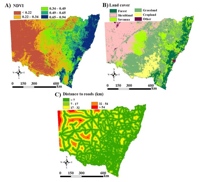
Fuel loads including the normalized difference vegetation index (NDVI) and land cover, and human-made factors such as distance to roads were
also used in this study. NDVI and land cover data (Figs. 4A and 4B) were collected from the USGS (MODIS 1-km MYD13A3 NDVI) (USGS 2021).
NDVI, which displays the coverage and density of surface vegetation in an image and land cover, is an element in the preservation of the
environment (Gigović et al. 2019). Land cover has been classified into six categories: forest, shrubland, savanna, grassland, cropland, and
others. The distance to roads was calculated using the Euclidean distance technique in ArcGIS (Fig. 4C). Distance to roads data were collected
from Open Street Map (OSM 2021). Finally, we considered eight conditioning factors for bushfire susceptibility mapping. They are slope, aspect,
elevation, annual mean precipitation, annual maximum temperature, NDVI, land cover, and distance to roads.
2.3. GEP
GEP is a population-based algorithm (similar to GA and genetic programming (GP)) introduced by Ferreira (Ferreira 2001). Individuals are
selected according to their fitness. One or more genetic operators have been used to bring genetic variation to the population (Ferreira 2001).
GEP can solve complex problems more quickly than GP (Nikraz 2011). Individuals are linear entities with fixed lengths in GEP, but they express
themselves in nonlinear expression trees (ETs) with different sizes (Nikraz 2011).
The GEP algorithm initiates with a population that is randomly generated (Ferreira 2001). Individuals are expressed and evaluated, and then are
chosen to reproduce based on their fitness (Ferreira 2001). The process of expression, selection, and reproduction is repeated until either a
determined number of generations or final solution for the problem is obtained (Ferreira 2001). The replication cannot bring variety to the
population, so that the algorithm needs other operators to introduce variation to the population (Ferreira 2001). Chromosomes are copied
without any changes in the replication step, but the rest of the operators select the chromosomes to conduct a particular modification (Ferreira
2001). Replication is necessary, but is an unexciting operator because it does not contribute to genetic diversity (Ferreira 2001). Other operators,
such as mutation, inversion, and recombination, have been used to vary the population. Mutations can occur anywhere on the chromosome
(Ferreira 2001). In mutation, head symbols are allowed to change to function or terminal, but terminals in tails have the option to be replaced by
terminals (Ferreira 2001; Ebtehaj et al. 2015). In inversion, a random sequence is selected in the chromosome’s head and inverted (Ebtehaj et al.
2015). In recombination, two chromosomes, which have been randomly selected, parent, combine with each other, and introduce two new
offspring to the generation (Ferreira 2001).
We selected a population size of 30 and chromosome head length of 12. In addition, five genes were linked to each chromosome (with addition
function). Bushfire conditioning factors and constants create a terminal set. The functions were selected by following the steps given in our
previous research (Hosseini and Lim 2021).
2.4. FR
FR is a statistical technique based on the correlation between the distribution of bushfire occurrence and bushfire conditioning factors (Lee et al.
2007; Razavizadeh et al. 2017; Aditian et al. 2018). In the FR approach, weight is assigned to each factor based on the contribution of each
factor to the bushfire occurrence (Razavizadeh et al. 2017). The FR for each class of conditioning factors is
BF (x)
T BF
(1)
FR = ,
N (x)
TN
where BF(x) is the number of bushfires occurring in each class x, TBF is the total number of bushfires, N(x) is the number of pixels for each class
x, and TN is the total number of pixels for the entire study area. Bushfire susceptibility mapping was created using the total weighted FR for the
factors (Dorji and Ongsomwang 2017). A higher FR implies a higher potential for bushfire susceptibility (Pradhan et al. 2015).
2.5. RF
The RF method introduced by Breiman (2001) is a strong and flexible ensemble learning methodology based on DT (Breiman 2001; Ahmad et al.
2017; Naghibi and Ahmadi 2017). The RF approach is suitable for nonlinear and high-dimensional problems, such as bushfire susceptibility
(Gigović et al. 2019). RF is trained with bootstraps and is tested with out-of-bag samples (Sarica et al. 2017). RF constructs trees based on
bootstrapped samples drawn randomly from the training dataset (Naghibi and Ahmadi 2017; Couronné et al. 2018). In the implementation of RF,
the number of trees (N_tree) and the number of variables for each split (N_try) are parameters that need to be adjusted (Naghibi and Ahmadi
2017; Noi and Kappas 2018). N_tree should be sufficiently large such that each conditioning factor has a sufficient probability to be selected.
N_try as a default is the square root of the number of conditioning factors for classification (Couronné et al. 2018; Gigović et al. 2019).
Page 4/14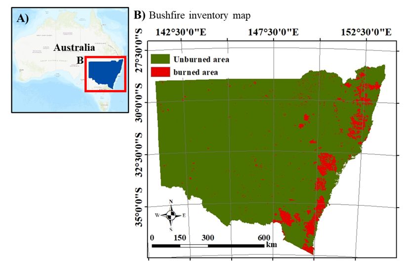
N_tree and N_try have been optimized to reduce errors and increase the accuracy (Gigović et al. 2019). In this study, we used the RF package in
the R open-source software (R Core Team 2020) with N_tree = 1,000 and N_try = 3.

One of the features of RF is the allowance of variable importance investigation (Gigović et al. 2019). The RF variable importance is calculated
using the Gini index (Sarica et al. 2017). The prediction power of conditioning factors based on the principle of impurity reduction is measured
by the Gini index in classification or regression (Sarica et al. 2017). Land cover was the most important factor, followed by precipitation and
NDVI in our study, based on variable importance.
2.6. SVM
SVM, introduced by Vapnik (1995), is a data-mining ML approach used to solve problems in different fields (Vapnik 1995; Gigović et al. 2019;
Jaafari and Pourghasemi 2019; Gholamnia et al. 2020). The SVM method is based on the risk minimization principle to separate two different
classes using a linear hyperplane (Gigović et al. 2019; Jaafari and Pourghasemi 2019). SVM generates a separating hyperplane and changes
the nonlinear problem to a linear problem (Jaafari and Pourghasemi 2019). The optimal hyperplane can be found when there are maximal
separations between the margins of the different classes of the problem (Gholamnia et al. 2020).

In SVM implementation, different kernel functions can be applied. RBF, polynomial, linear, and sigmoid kernels are the most common kernels
used in SVM classification (Gigović et al. 2019). We used RBF as a kernel function for bushfire susceptibility mapping. The performance of the
SVM model depends on two parameters, the kernel width (γ) and regularization constant (C), which should be adjusted properly (Gigović et al.
2019). We tuned the data to find the best values for γ and C for the model using the R open-source software.
2.7. LR
LR is a widely used approach for the natural hazard prediction (Hong et al. 2019). In bushfire modeling, LR creates a statistical relationship
between the independent variable (bushfire occurrence) and dependent variables (conditioning factors) to determine the most accurate model to
produce the probability of fire occurrence (Hong et al. 2019). LR uses Eq. (2) to find the best-fit model (Hong et al. 2019),

                                                                                                    (2)
                                                   Z = b0 + b1 x1 + b2 x2 + ⋯ + bn xn .

where Z represents the existence or absence of bushfire, b0 is an equation intercept, b1, b2, …, bn are the model coefficients, and xi’s refer to the
conditioning factors (Hong et al. 2019).

The probability of fire occurrence obtained by LR in each pixel can be expressed as (Hong et al. 2019)

                                                                     p =   ,
                                                                           1
                                                                           1+e
                                                                               (3)
                                                                              −z

where p is the probability of fire occurrence (between 0 and 1) (Hong et al. 2019).

2.8. Ensemble methods
In this study, we proposed four ensemble techniques: GEPFR, RFFR, SVMFR, and LRFR. In these methods, we classified the different conditioning
factors. Weights for different classes were calculated using the FR. Maps of different classes of each factor were obtained using ArcGIS. The
results were introduced as inputs to GEP, RF, SVM, and LR. Finally, the output was mapped in ArcGIS for GEPFR, RFFR, SVMFR, and LRFR.

3. Results And Validation
We generated the bushfire susceptibility map using ensemble techniques including GEPFR, RFFR, SVMFR, and LRFR and individual methods
such as GEP, RF, SVM, and FR. The area under the curve (AUC) of the receiver operating characteristic (ROC) and accuracy were used to evaluate
the models. ROC is a nondependent threshold method commonly used to evaluate bushfire susceptibility models (Gigović et al. 2019). Accuracy
is defined as a ratio of cases classified correctly to the total data (Hoang and Tien Bui 2018). Accuracy is another common quality metric
between different models, calculated by

                                                                               T P +T
                                                                                     (4)
                                                                                   +T N
                                                                                      N +F P +F N
                                                                Accuracy =     ,P
                                                                               T

where false positive (FP) represents the number of pixels incorrectly classified as fire class, true negative (TN) represents the number of pixels
correctly classified as nonfire class, true positive (TP) represents the number of pixels correctly determined as fire class, and false negative (FN)
represents the number of pixels incorrectly classified as nonfire class (Hong et al. 2019).

                                                                      Page 5/14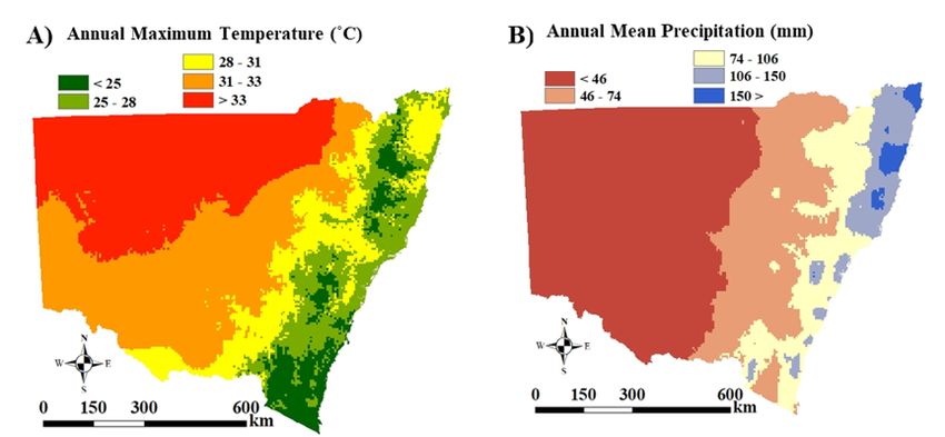
The mathematical formula generated from GeneExproTools by GEPFR is
                                                    (d +d )
                                                    +α
                                                    2 1  2
                                                                                                                            (5)
                                 (d +d )
                         F = ( 2)4 × 3log (d3 ) +   2+   log (d6 ) + (d       × d5 ) + d7 × arctan(d       − β + 2γ+d7 ),
                                                                          7                            6

                         α = 7.52, β = −5.83, γ = 7.05,

where d1 is the slope, d2 is the altitude, d3 is the NDVI, d4 is the distance to road, d5 is the land cover, d6 is the annual maximum temperature, and
d7 is the annual mean precipitation.

The bushfire susceptibility map generated by the GEPFR is presented in Fig. 5A. The majority of the study area was categorized as having a very
low possibility of bushfire using the GEPFR method. The coastal area is covered by moderate to very high possibility of bushfire, while the
western area has a very low possibility of bushfire. The AUCs of the GEPFR model in the training and testing sets were 0.892 and 0.890, while
the accuracies were 92.45% and 92.69%, respectively (Table 1).

We also generated a bushfire susceptibility map using the RFFR model (Fig. 5B), which similarly labeled the majority of the study area as having
a very low possibility of bushfire. The northeastern, eastern, and southeastern parts of NSW were predicted to have a very high potential for
bushfires. The RFFR model had an AUC of 0.895 for the training set and 0.875 for the testing set. The accuracies for training and testing were
95.29% and 94.70%, respectively (Table 1).

The majority of the map was covered by a low possibility of bushfire in the susceptibility map generated by SVMFR (Fig. 5C). The northeast,
east, and southeast were covered by a very high possibility of bushfires, but SVMFR was not successful in finding areas with a high potential for
bushfires in the study area. SVMFR had AUCs of 0.796 and 0.753 and accuracies of 94.54% and 94.28% in the training and testing sets,
respectively (Table 1).

The bushfire susceptibility map generated by LRFR (Fig. 5D) shows that the west and central parts of NSW have very low possibility of bushfire.
The northeast, east, and southeast exhibited moderate to very high potential for bushfires. The AUCs for the training and testing sets were 0.890
and 0.887, respectively. The accuracies in the training and testing sets were 93.50% and 93.67%, respectively (Table 1). The model generated by
LRFR is

                                                                                                                                                 (6)
 z = −5.039 + 0.143 × A + 0.169 × S − 0.170 × E + 0.074 × N + 0.028 × D + 0.274 × L − 0.273 × T + 0.338 × P

where A is aspect, S is slope, E is elevation, N is NDVI, D is distance to road, L is land cover, T is annual maximum temperature, and P is annual
mean precipitation.

Individual methods were also used to generate susceptibility maps to compare their results with those of ensemble methods. The individual
methods included GEP, RF, SVM, and FR.

The bushfire model generated by GEP (Fig. 6A) shows that the study area is mostly covered by a low possibility of bushfire in the western and
central parts of NSW. The northeast, east, and southeast are covered by a moderate to very high possibility for bushfires. GEP had AUCs of 0.884
and 0.882 for the training and testing sets, respectively. The accuracies of the GEP model in the training and testing phases were 91.92% and
91.89%, respectively (Table 1).

The bushfire map generated by RF (Fig. 6B) in the central and western parts shows a very low possibility of bushfire, while smaller areas in the
northeast, east, and southeast are categorized with very high possibilities for bushfires. RF had AUCs of 0.902 and 0.876 in the training and
testing sets, while the accuracies were 95.47% and 94.51%, respectively (Table 1).

We also generated a bushfire susceptibility map using SVM (Fig. 6C), which is similar to the map generated by SVMFR. The majority of the
study area is categorized as low-possibility class for bushfires. The northeast, east, and southeast are covered by a very high potential for
bushfires. SVM had AUCs of 0.868 and 0.781 in the training and testing sets, respectively. The SVM had accuracies of 96.03% and 94.21% in the
training and testing sets, respectively (Table 1). Similar to SVMFR, this method is not successful in finding areas with a high potential for
bushfire occurrence.

The bushfire susceptibility map generated by FR (Fig. 6D) shows a very low potential in the west and low possibilities in the central NSW. The
northeast, east, and southeast of the area are covered by moderate to very high potential for bushfires. FR had an AUC of 0.888 and accuracy of
87.20% (Table 1).

                                                                      Page 6/14
Table 1
Comparison of parameters for
different methods.
Method AUC Accuracy (%)
GEPFR 0.890 92.69
RFFR 0.875 94.70
SVMFR 0.753 94.28
LRFR 0.887 93.67
GEP 0.882 91.89
RF 0.876 94.51
SVM 0.781 94.21
FR 0.888 87.20
The generated bushfire susceptibility maps (from different individual and ensemble methods) were reclassified using the natural break
classification method. Finally, the generated maps were categorized into five different subclasses (very low, low, moderate, high, and very high).
The west and central areas of NSW were categorized with very low to low possibility for bushfire in all maps generated by different individual
and ensemble methods. The northeast, east, and southeast of NSW in different methods have moderate to very high potential for bushfires. The
bushfire susceptibility maps generated by RF and RFFR categorized the majority of the area into two categories: very low and very high; however,
the other methods allocated areas in all five possibility classes.
4. Discussion
We presented a GEPFR approach for modeling bushfires in NSW, Australia. The majority of bushfires occurred in the eastern, northeastern, and
southeastern regions of NSW, possibly due to the high vegetation and forest in those areas. Our findings showed that the land cover and
precipitation had significant impacts on the occurrence of bushfires. Bushfires are more common in particular land cover types, such as native
forests and grazing lands (Deb et al. 2020). Another study also showed that forests had the highest potential for fire occurrence among land
covers due to the availability of massive loads of fuel (Zhang et al. 2015).
The majority of bushfires are located in mountainous and coastal regions in our study area. Previous studies also demonstrated that
mountainous and coastal areas have a high potential for bushfire occurrence (Zhang et al. 2015; Sun et al. 2016).
The annual mean precipitation was highest in the eastern part of NSW, compared to the western and central parts of NSW. The annual mean
precipitation is one of the most important factors in our study area. Our results showed that the precipitation had a strong positive correlation
with the bushfire occurrence. Similarly, a previous study has shown that the precipitation increases the amount of vegetation, resulting in a
higher risk of flammability (Collins et al. 2014). A positive correlation between bushfires and precipitation was also reported in southeastern
Arizona, which indicates the availability of higher fuel loads as a result of a higher precipitation (Crimmins and Comrie 2005; Nicholls and Lucas
2007). The precipitation can increase the moisture content, which is expected to reduce the bushfire occurrence. On a large scale, the
precipitation can increase the available fuel for bushfires, which is the reason for the positive correlation between the bushfire occurrence and
precipitation (Zhang et al. 2015). Another study also showed a substantial positive nonlinear association between cumulative antecedent
rainfall (over several years) and occurrence of fires in central Australia (Nicholls and Lucas 2007; Griffin 2017). Similarly, widespread wildfires in
northern Australia occurred after periods of above-average rainfall (Felderhof and Gillieson 2006; Nicholls and Lucas 2007).
In NSW, the temperature is higher in the central and western parts. However, our results indicate that these regions have a low probability of
bushfire. The western and central parts also have the highest temperature and lowest annual precipitation rate. As a result, the fuel load in these
areas is lower than those in other areas. This could be the reason for the classification of the western areas of NSW with a low possibility for
bushfires.
Our results show that forest-covered areas have a moderate to high probability of bushfires in the generated prediction maps. The area with a
low potential is mostly covered by shrublands and grasslands. Similarly, other studies have shown that the forest land cover has a strong
positive correlation with bushfire occurrence, whereas the lowest bushfire probability belonged to shrublands (Zhang et al. 2016).
The comparison of the maps created by different methods show that the GEPFR method has the highest AUC, while the others have almost the
same AUCs except SVM and SVMFR which have the lowest AUCs. The predictions by RFFR and RF are similar. They categorized the data in
Page 7/14almost two groups, while GEPFR, LRFR, GEP and FR classified the data in various classes with very low to very high potential of bushfire. The
maps obtained by SVM and SVMFR are almost the same, but the map generated by SVM has a higher AUC. GEPFR allocated the majority of the
study area to very low potential for bushfire, while GEP categorized the majority of the study area with a low potential for bushfire. GEPFR, RFFR,
and LRFR determined that land cover and precipitation were the most important factors in bushfire susceptibility mapping.
5. Concluding Remarks
In this study, we applied eight different methods, including ensemble methods of GEPFR, RFFR, SVMFR, and LRFR and individual methods such
as GEP, RF, SVM, and FR, for bushfire susceptibility mapping in NSW, Australia. Historical bushfire data between 2010 and 2020 were collected to
create a bushfire inventory map. Eight conditioning factors were used to generate bushfire susceptibility maps across NSW. The prediction
models showed that the eastern, northeastern, and southeastern parts of NSW had the highest probability of bushfires, which are mostly covered
by forest. In contrast, the western and central parts of the study area have a very low potential in the bushfire susceptibility mapping, while these
areas have the highest temperature and lowest precipitation. The western and central parts of NSW are also covered with shrublands,
grasslands, and croplands. The generated maps were evaluated based on their AUCs. GEPFR was the best method for the prediction of bushfires
in NSW, Australia. GEPFR is a user-friendly method and thus suitable for the prediction of bushfires in different bushfire-prone areas.
Declarations
Not applicable.
Description of author's responsibilities
Maryamsadat Hosseini: Conceptualization, Data collection, Data analyses, Methodology, Software, Visualization, Writing - original draft,
Reviewing & editing. Samsung Lim: Supervision, Conceptualization, Writing, Critical reviewing and editing.
References
1. Aditian A, Kubota T, Shinohara Y (2018) Geomorphology Comparison of GIS-based landslide susceptibility models using frequency ratio ,
logistic regression , and artificial neural network in a tertiary region of Ambon , Indonesia. Geomorphology 318:101–111.
https://doi.org/10.1016/j.geomorph.2018.06.006
2. Ahmad MW, Mourshed M, Rezgui Y (2017) Trees vs Neurons : Comparison between random forest and ANN for high-resolution prediction of
building energy consumption. Energy Build 147:77–89. https://doi.org/10.1016/j.enbuild.2017.04.038
3. BOM (2021) Australia’s official weather forecasts and weather radar - Bureau of Meteorology. http://www.bom.gov.au/. Accessed 8 Mar
2021
4. Breiman LEO (2001) Random Forests. Mach Learn 45:5–32. https://doi.org/10.1023/A:1010933404324
5. Bui DT, Le KTT, Nguyen VC, et al (2016) Tropical forest fire susceptibility mapping at the Cat Ba National Park area, Hai Phong City, Vietnam,
using GIS-based Kernel logistic regression. Remote Sens 8:1–15. https://doi.org/10.3390/rs8040347
6. Cao Y, Wang M, Liu K (2017) Wildfire Susceptibility Assessment in Southern China: A Comparison of Multiple Methods. Int J Disaster Risk
Sci 8:164–181. https://doi.org/10.1007/s13753-017-0129-6
7. Collins L, Bradstock RA, Penman TD (2014) Can precipitation influence landscape controls on wildfire severity’ A case study within
temperate eucalypt forests of south-eastern Australia. Int J Wildl Fire 23:9–20. https://doi.org/10.1071/WF12184
8. Couronné R, Probst P, Boulesteix AL (2018) Random forest versus logistic regression: A large-scale benchmark experiment. BMC
Bioinformatics 19:1–14. https://doi.org/10.1186/s12859-018-2264-5
9. Crimmins MA, Comrie AC (2005) Interactions between antecedent climate and wildfire variability across south-eastern Arizona. Int J Wildl
Fire 13:455–466
10. Deb P, Moradkhani H, Abbaszadeh P (2020) Causes of the Widespread 2019 – 2020 Australian Bush fi re Season Earth ’ s Future.
https://doi.org/10.1029/2020EF001671
11. Dorji S, Ongsomwang S (2017) Wildfire Susceptibility Mapping in Bhutan Using Geoinformatics Technology. Suranaree J Sci Technol
24:213–237
12. Ebtehaj I, Bonakdari H, Hossein A, et al (2015) Gene expression programming to predict the discharge coefficient in rectangular side weirs.
Appl Soft Comput J 35:618–628. https://doi.org/10.1016/j.asoc.2015.07.003
13. Emamgolizadeh S, Bateni SM, Shahsavani D, et al (2015) Estimation of soil cation exchange capacity using Genetic Expression
Programming (GEP) and Multivariate Adaptive Regression Splines (MARS). J Hydrol 529:1590–1600.
https://doi.org/10.1016/j.jhydrol.2015.08.025
Page 8/1414. Eskandari S, Amiri M, Sãdhasivam N, Pourghasemi HR (2020) Comparison of new individual and hybrid machine learning algorithms for
modeling and mapping fire hazard: a supplementary analysis of fire hazard in different counties of Golestan Province in Iran. Nat Hazards
104:305–327. https://doi.org/10.1007/s11069-020-04169-4
15. Felderhof L, Gillieson D (2006) Comparison of fire patterns and fire frequency in two tropical savanna bioregions. 736–746.
https://doi.org/10.1111/j.1442-9993.2006.01645.x
16. Ferreira C (2001) Gene expression programming: a new adaptive algorithm for solving problems. arXiv Prepr cs/0102027
17. Gholamnia K, Gudiyangada Nachappa T, Ghorbanzadeh O, Blaschke T (2020) Comparisons of diverse machine learning approaches for
wildfire susceptibility mapping. Symmetry (Basel) 12:604
18. Ghorbanzadeh O, Kamran KV, Blaschke T, et al (2019) Spatial prediction of wildfire susceptibility using field survey gps data and machine
learning approaches. Fire 2:1–23. https://doi.org/10.3390/fire2030043
19. Gigović L, Pourghasemi HR, Drobnjak S, Bai S (2019) Testing a new ensemble model based on SVM and random forest in forest fire
susceptibility assessment and its mapping in Serbia’s Tara National Park. Forests 10:. https://doi.org/10.3390/f10050408
20. Griffin GF (2017) Wildfires in the central Australian rangelands , 1970-1980 . 1970–1980
21. Hoang ND, Tien Bui D (2018) Spatial prediction of rainfall-induced shallow landslides using gene expression programming integrated with
GIS: a case study in Vietnam. Nat Hazards 92:1871–1887. https://doi.org/10.1007/s11069-018-3286-z
22. Hong H, Jaafari A, Zenner EK (2019) Predicting spatial patterns of wildfire susceptibility in the Huichang County, China: An integrated model
to analysis of landscape indicators. Ecol Indic 101:878–891. https://doi.org/10.1016/j.ecolind.2019.01.056
23. Hong H, Naghibi SA, Moradi Dashtpagerdi M, et al (2017) A comparative assessment between linear and quadratic discriminant analyses
(LDA-QDA) with frequency ratio and weights-of-evidence models for forest fire susceptibility mapping in China. Arab J Geosci 10:.
https://doi.org/10.1007/s12517-017-2905-4
24. Hosseini M, Lim S (2021) Gene expression programming and ensemble methods for bushfire susceptibility mapping: a case study of
Victoria, Australia. Geomatics, Nat Hazards Risk 12:2367–2386. https://doi.org/10.1080/19475705.2021.1964618
25. Jaafari A, Gholami DM, Zenner EK (2017) A Bayesian modeling of wildfire probability in the Zagros Mountains, Iran. Ecol Inform 39:32–44.
https://doi.org/10.1016/j.ecoinf.2017.03.003
26. Jaafari A, Mafi-Gholami D, Thai Pham B, Tien Bui D (2019) Wildfire Probability Mapping: Bivariate vs. Multivariate Statistics. Remote Sens
11:618. https://doi.org/10.3390/rs11060618
27. Jaafari A, Pourghasemi HR (2019) Factors Influencing Regional-Scale Wildfire Probability in Iran. In: Spatial Modeling in GIS and R for Earth
and Environmental Sciences. Elsevier, pp 607–619
28. Jain P, Coogan SCP, Subramanian SG, et al (2020) A review of machine learning applications in wildfire science and management. arXiv
Prepr arXiv200300646
29. Kayadelen C (2011) Soil liquefaction modeling by Genetic Expression Programming and Neuro-Fuzzy. Expert Syst Appl 38:4080–4087.
https://doi.org/10.1016/j.eswa.2010.09.071
30. Lee S, Pradhan B, Article O (2007) Landslide hazard mapping at Selangor, Malaysia using frequency ratio and logistic regression models.
Landslides 4:33–41. https://doi.org/10.1007/s10346-006-0047-y
31. Leuenberger M, Parente J, Tonini M, et al (2018) Wildfire susceptibility mapping: Deterministic vs. stochastic approaches. Environ Model
Softw 101:194–203
32. Ma J, Cheng JCP, Jiang F, et al (2020) Advanced Engineering Informatics Real-time detection of wildfire risk caused by powerline vegetation
faults using advanced machine learning techniques. Adv Eng Informatics 44:101070. https://doi.org/10.1016/j.aei.2020.101070
33. Milton LA, White AR (2020) Neurochemistry International The potential impact of bushfire smoke on brain health. Neurochem Int
139:104796. https://doi.org/10.1016/j.neuint.2020.104796
34. Mousavi SM, Aminian P, Gandomi AH, et al (2012) A new predictive model for compressive strength of HPC using gene expression
programming. Adv Eng Softw 45:105–114. https://doi.org/10.1016/j.advengsoft.2011.09.014
35. Naghibi SA, Ahmadi K (2017) Application of Support Vector Machine , Random Forest , and Genetic Algorithm Optimized Random Forest
Models in Groundwater Potential Mapping. 2761–2775. https://doi.org/10.1007/s11269-017-1660-3
36. Nami MH, Jaafari A, Fallah M, Nabiuni S (2018) Spatial prediction of wildfire probability in the Hyrcanian ecoregion using evidential belief
function model and GIS. Int J Environ Sci Technol 15:373–384. https://doi.org/10.1007/s13762-017-1371-6
37. Nicholls N, Lucas C (2007) Interannual variations of area burnt in Tasmanian bushfires: Relationships with climate and predictability. Int J
Wildl Fire 16:540–546. https://doi.org/10.1071/WF06125
38. Nikraz IAH (2011) Correlation of Pile Axial Capacity and CPT Data Using Gene Expression Programming. 725–748.
https://doi.org/10.1007/s10706-011-9413-1
Page 9/1439. Noi PT, Kappas M (2018) Comparison of Random Forest, k-Nearest Neighbor, and Support Vector Machine Classifiers for Land Cover
Classification Using Sentinel-2 Imagery. https://doi.org/10.3390/s18010018
40. OSM (2021) OpenStreetMap. https://www.openstreetmap.org/#map=4/-28.15/133.28. Accessed 8 Mar 2021
41. Pham BT, Jaafari A, Avand M, et al (2020) Performance evaluation of machine learning methods for forest fire modeling and prediction.
Symmetry (Basel) 12:. https://doi.org/10.3390/SYM12061022
42. Pourghasemi HR (2016) GIS-based forest fire susceptibility mapping in Iran: a comparison between evidential belief function and binary
logistic regression models. Scand J For Res 31:80–98
43. Pourtaghi ZS, Pourghasemi HR, Rossi M (2015) Forest fire susceptibility mapping in the Minudasht forests, Golestan province, Iran. Environ
Earth Sci 73:1515–1533. https://doi.org/10.1007/s12665-014-3502-4
44. Pradhan B, Dini M, Bin H (2015) Forest fire susceptibility and risk mapping using remote sensing and geographical information systems (
GIS ). https://doi.org/10.1108/09653560710758297
45. Pradhan B, Suliman MDH Bin, Awang MA Bin (2007) Forest fire susceptibility and risk mapping using remote sensing and geographical
information systems (GIS). Disaster Prev Manag An Int J 16:344–352. https://doi.org/10.1108/09653560710758297
46. R Core Team (2020) R: A language and environment for statistical computing. R Foundation for Statistical Computing, Vienna, Austria
47. Razavi-Termeh SV, Sadeghi-Niaraki A, Choi SM (2020) Ubiquitous GIS-based forest fire susceptibility mapping using artificial intelligence
methods. Remote Sens 12:. https://doi.org/10.3390/rs12101689
48. Razavizadeh S, Solaimani K, Massironi M (2017) Mapping landslide susceptibility with frequency ratio , statistical index , and weights of
evidence models : a case study in northern Iran. Environ Earth Sci 76:1–16. https://doi.org/10.1007/s12665-017-6839-7
49. Sachdeva S, Bhatia T, Verma AK (2018) GIS-based evolutionary optimized Gradient Boosted Decision Trees for forest fire susceptibility
mapping. Nat Hazards 92:1399–1418. https://doi.org/10.1007/s11069-018-3256-5
50. Sarica A, Cerasa A, Quattrone A (2017) Random forest algorithm for the classification of neuroimaging data in Alzheimer’s disease: A
systematic review. Front Aging Neurosci 9:1–12. https://doi.org/10.3389/fnagi.2017.00329
51. Sun L, Trinder J, Rizos C (2016) Proceedings for the 5th International Fire Behavior and Fuels Conference April 11-15, 2016, Portland,
Oregon, USA Published by the International Association of Wildland Fire, Missoula, Montana, USA. In: The 5th International Fire Behavior
and Fuels Conference
52. Tehrany MS, Özener H, Kalantar B, et al (2021) Application of an Ensemble Statistical Approach in Spatial Predictions of Bushfire
Probability and Risk Mapping. 2021:
53. Tonini M, D’andrea M, Biondi G, et al (2020) A machine learning-based approach for wildfire susceptibility mapping. The case study of the
liguria region in italy. Geosci 10:. https://doi.org/10.3390/geosciences10030105
54. USGS (2021) EarthExplorer. https://earthexplorer.usgs.gov/. Accessed 8 Mar 2021
55. Vapnik V (1995) The Nature of Statistical Learning Theory. Springer, New York, NY
56. You W, Lin L, Wu L, et al (2017) Geographical information system-based forest fire risk assessment integrating national forest inventory
data and analysis of its spatiotemporal variability. Ecol Indic 77:176–184. https://doi.org/10.1016/j.ecolind.2017.01.042
57. Yu P, Xu R, Abramson MJ, et al (2020) Comment Bushfires in Australia : a serious health emergency under climate change. Lancet Planet
Heal 4:e7–e8. https://doi.org/10.1016/S2542-5196(19)30267-0
58. Zakaria NA, Azamathulla HM, Chang CK, Ghani AA (2010) Gene expression programming for total bed material load estimation-a case
study. Sci Total Environ 408:5078–5085. https://doi.org/10.1016/j.scitotenv.2010.07.048
59. Zhang G, Wang M, Liu K (2019) Forest Fire Susceptibility Modeling Using a Convolutional Neural Network for Yunnan Province of China. Int
J Disaster Risk Sci 10:386–403. https://doi.org/10.1007/s13753-019-00233-1
60. Zhang Y, Lim S, Sharples JJ (2015) Development of spatial models for bushfire occurrence in South-Eastern Australia. 326–332
61. Zhang Y, Lim S, Sharples JJ (2016) Modelling spatial patterns of wildfire occurrence in South-Eastern Australia. Geomatics, Nat Hazards
Risk 7:1800–1815. https://doi.org/10.1080/19475705.2016.1155501
Figures
Page 10/14Figure 1
Map of the study area. A) Australia and the location of NSW and B) a bushfire inventory map for NSW in the period of 2010 to 2020. Dark green
and red indicate unburned and burned areas, respectively.
Figure 2
Page 11/14Maps of topographic factors for NSW. A) Elevation, B) aspect, C) slope. The legend describes the color code for each map.
Figure 3
Maps of climate factors for NSW. A) Annual maximum temperature, B) annual mean precipitation. The legend describes the color code for each
map.
Figure 4
Maps of fuel load and human activity factors for NSW. A) NDVI, B) land cover, and C) distance to roads
Page 12/14Figure 5
Bushfire susceptibility mapping using ensemble methods. A) GEPFR, B) RFFR, C) SVMFR, and D) LRFR. The spectrum of dark green (very low) to
red (very high) represents the probability of bushfire.
Page 13/14Figure 6
Bushfire susceptibility mapping using single methods. A) GEP, B) RF, C) SVM, and D) FR. The spectrum of dark green (very low) to red (very high)
represents the probability of bushfire
Page 14/14You can also read