Global Warming Acceleration

Fig. 1. Global surface temperature anomalies (relative to 1880-1920) in 2016 and 2020.

                           Global Warming Acceleration
                                                                               14 December 2020
                                 James Hansen and Makiko Sato
Abstract. Record global temperature in 2020, despite a strong La Niña in recent months,
reaffirms a global warming acceleration that is too large to be unforced noise – it implies
an increased growth rate of the total global climate forcing and Earth’s energy imbalance.
Growth of measured forcings (greenhouse gases plus solar irradiance) decreased during
the period of increased warming, implying that atmospheric aerosols probably decreased in
the past decade. There is a need for accurate aerosol measurements and improved
monitoring of Earth’s energy imbalance.
November 2020 was the warmest November in the period of instrumental data, thus jumping
2020 ahead of 2016 in the 11-month averages (Fig. 1). December 2016 was relatively cool, so it
is clear that 2020 will slightly edge 2016 for the warmest year, at least in the GISTEMP analysis.
The rate of global warming accelerated in the past 6-7 years (Fig. 2). The deviation of the 5-year
(60 month) running mean from the linear warming rate is large and persistent; it implies an
increase in the net climate forcing and Earth’s energy imbalance, which drive global warming.

          Fig. 2. Global temperature and Niño3.4 Index through November 2020.

Fig. 3. Annual growth of GHG climate forcing (red is trace gases, mainly CFCs).

Variability of the 12-month running mean about the linear warming trend in the past 50 years is
mainly unforced variability associated with ENSO (El Niño Southern Oscillation). The two
largest deviations of the 60-month (5-year) running mean are forced deviations. The 1980s
bump is from the CFC bump in the greenhouse gas (GHG) climate forcing growth (Fig. 3). The
early-mid 1990s valley is the cooling due to the volcano of the century (Mt. Pinatubo).
The GHG climate forcing growth rate has accelerated in the past decade (Fig. 3), but not enough
to account for the observed acceleration of the global warming rate. The validity of this
conclusion becomes clearer when we look at the total measured climate forcing – the black curve
in Fig. 4 – which is the sum of the GHG and solar climate forcings. During the period of global
warming acceleration – 2015-2020 – the climate forcing growth rate due to measured forcings
was a minimum.
Global warming is driven both by Earth’s current energy imbalance and by the recent growth of
net climate forcing. The most recent several years have the largest effect on current warming.
Even if you are not a physicist or mathematician, this is easy to understand – and by taking the
trouble to understand, you can say that you understand Sir Isaac Newton’s calculus.

 Fig. 4. Black curve is the net annual change of measured climate forcings, GHGs + Solar.

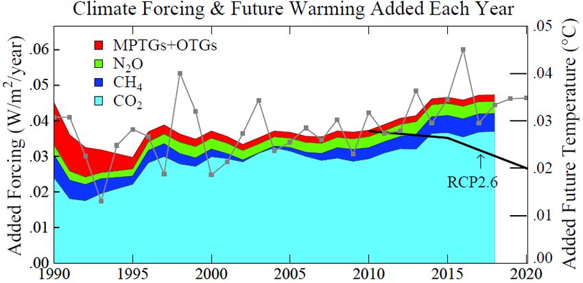
Figure 5. Climate model’s response function: fraction of the final response versus time. In
the graph on the right the first 100 years are expanded with a log scale for remaining years.

Fig. 5 shows the response function for GISS model E-R based on a 2000 year run for an instant
CO2 doubling with fixed ice sheets, vegetation distribution, and other long-lived GHGs. The
expanded time scale for the first 100 years in the graph on the right shows that about a third of
the response is obtained within the first 5 years. The remaining 2/3 is recalcitrant (slow).
The climate response function, R(t), is the fraction (%) of equilibrium surface temperature
response to an applied forcing as a function of time. Expected global temperature change is the
forcing added this year times response function for year 1, plus forcing added last year times the
response function for year 2, plus the forcing added the year prior times the response function for
year 3… You get the idea. In equation form we write
                                     T(t) = ʃ S R(t) [dF/dt] dt,
where T(t) is temperature anomaly at time t, S is climate sensitivity (~¾°C per W/m2), R(t) is the
response function at year t, and dF/dt is the forcing added in year t. dt is just one year if you are
adding up the pieces in one-year blocks – with a computer, we let dt be smaller. This simple
calculation is very accurate (Hansen, 2008) as long as the ocean overturning circulation does not
shut down, in which case you need a full atmosphere-ocean model.
We are showing the response function to explain how we know that if the only forcing changes
were the GHGs and the Sun (black curve in Fig. 4) there would be no acceleration of global
warming in the past five years – indeed, there should be a decrease in the warming rate. The
real-world acceleration tells us that there must be another forcing, which is unmeasured. There
is only one good candidate: aerosols. Although NASA chose not to measure the aerosol climate
forcing (Chapter 33 of Sophie’s Planet), some aerosol models suggest that global aerosol amount
has decreased in the past decade (Bauer et al., 2020).
BTW, the enquiring mind is probably saying “well if the forcing change in the past five years is
expected to leave a significant signature, should we not expect the solar cycle to show up in
observed global temperature?” Indeed, the solar curve (yellow curve in Fig. 4) and observed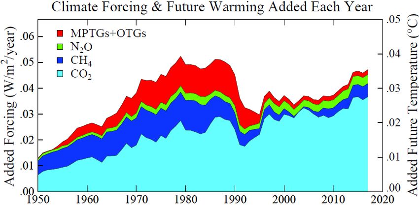

Figure 6. Chart 20 of Bjerknes lecture (Hansen, 2008).

global temperature curve have maximum correlation of 47% with temperature lagging the solar
forcing by 1-2 years. If Earth were an all-land planet the lag should be ~0 years; if an all-ocean
planet the lag would be ~ quarter of the solar cycle, i.e., ~3 years; in the real world it should be
1-2 years. So, it works out right, despite the large volcanoes in that period.
How large is the aerosol forcing? In recent IPCC reports the GCMs (global climate models)
tended to use aerosol forcings in the range -0.5 W/m2 to -1.0 W/m2, despite the fact that the
IPCC radiative forcing chapters suggest a larger (more negative) aerosol forcing, with a direct
aerosol forcing ~ -0.5 W/m2 and an indirect aerosol forcing (via cloud effects) ~ -1 W/m2, with
large uncertainty bars. Consistent with the radiative forcing chapters, we (Hansen et al, 2011)
made a strong case that the actual aerosol forcing is -1.6 ±0.3 W/m2. We also infer why most
GCMs (including the GISS model) “need” a smaller aerosol effect – if they want to match
observed global warming in the past century. The reason is that the models mix heat too
efficiently into the ocean – so to match observed warming the models need a larger net forcing,
which they achieve by omitting some of the negative aerosol forcing.
Is this important? Yes. It means that the little blip of extra warming that we got in the past five
years is only a down payment on the penalty that young people will pay for our Faustian bargain.
Mephistopheles is coming, but it is our grandchildren that he will be dragging off.

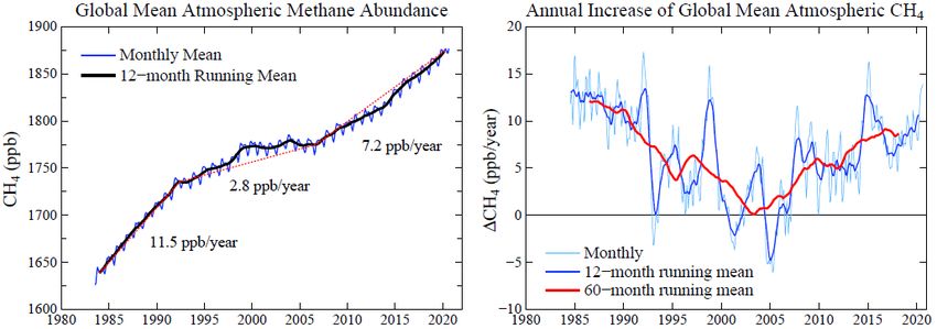
Figure 7. CO2, CH4 and N2O amounts and growth rates.

Note that the current GCM modeling associated with IPCC, CMIP6 models, include model
responses to instantaneous forcing (Smith et al., 2020). It will be possible to infer response
functions of different models, and it should be easier to interpret model results.

Aerosol summary.       Continued ignorance of the aerosol climate forcing, given the importance
of aerosols for future climate change, should be unacceptable. The required measurements need
to define the aerosol and cloud particle microphysics in detail. We know how to achieve that

Figure 8. Annual growth of GHG climate forcing (red is trace gases, mainly CFCs).

detail – it requires multi-spectral, multi-angle, polarimetric observations of reflected sunlight
from space with the polarization measured to an accuracy ~0.1 percent (Mishchenko et al.,
2007). There should be a dedicated small satellite monitoring program to quantify and monitor
the aerosol direct and indirect climate forcings. This is one of the handful of essential
measurement – which include GHGs, Earth’s gravity field, and Earth’s energy imbalance – that
are needed to interpret climate change and impacts. Earth’s energy imbalance requires
maintenance and improvements to the Argo float observations, especially in the regions around
the Antarctic ice shelves (von Schuckmann et al., 2020).

How are greenhouse gas forcings doing, up-to-date?         Are growth rates starting to decline?
Not exactly – see Fig. 7. CO2 growth is down a bit this year, and it should go down substantially
in 2021, as the expected response to the strong La Niña now underway. CH4 growth rate is
shooting up, presumably as a result of “fracking,” increased venting at oil wells, and global
warming feedbacks from warming wetlands and permafrost. N2O growth rate continues to
increase slowly (the oscillations in growth rate presumably are variability of the stratospheric
sink, related to stratospheric dynamics and stratosphere-troposphere exchange).
Slower CO2 growth offsets increased CH4 and N2O growth, so our estimate for the added GHG
forcing in 2020 is essentially the same as in 2019. The annual forcing increase is shown by the
dots on the gray line in Fig. 8. We use the 5-year running mean (in Fig. 3 and Fig. 8) for the
colored portion of the chart to minimize oscillatory changes.
Note that the gap continues to grow between the actual growth of GHG forcing and the RCP2.6
scenario that would keep global warming to about 1.5°C. As discussed in our “Young People’s
Burden” paper (Hansen et al. 2017), the cost of CO2 removal to get back on track is likely to be
in the trillions of dollars.

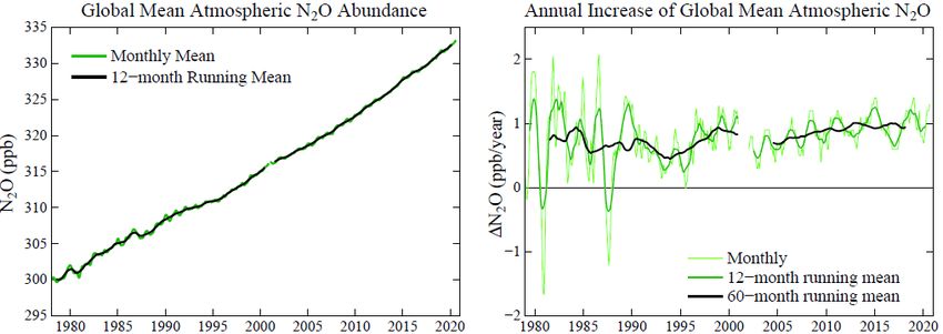
Figure 9. Global temperature anomalies in the first 11 months of each of the past six years.

Temperature maps. Siberia and the Arctic Ocean had the largest warm anomalies in 2020, but
it was warmer than the 1951-1980 average almost everywhere (Fig. 9). The global maps employ
1951-1980 as base period so that good global coverage of data is available for the base period.

One more thing.      Remember the cry of the climate deniers? Many of them were counting on
the Sun to go into a new, prolonged Maunder Minimum. That was possible, although the
resulting negative climate forcing (cooling) would be small compared with the human-made
GHG forcing.
It turns out that, on the contrary, we are now entering the next solar cycle. Solar minimum was
late 2019. The uptick in irradiance is small so far, but the predictions from some solar models
are that the coming maximum will be a strong one.
The impact of solar irradiance on global temperature lags solar irradiance by 1-2 years, so we are
still at the point where we are getting maximum cooling from the solar cycle. Maximum added
push of the solar cycle toward a warmer climate will be in mid-decade, i.e., in about 5 years.
Global temperature prognostication: 2021 will be cooler than 2020, because of the lagged effect
of the current strong La Niña. When the next El Niño occurs, perhaps about mid-decade, hang
onto your hat. Global emissions of GHGs had better be trending down by then!

Fig. 10. Satellite measured solar irradiance (top 2 panels) and sunspot numbers. Solar
minimum occurred in 2019.

You can sign up for our monthly global temperature updates here.
You can sign up for Hansen’s other Communications here.
                                                    References
Bauer, S.E., K. Tsigaridis, G. Fulavegi, M. Kelley, K.K. Lo, R.L. Miller, L. Nazarenko, G.A. Schmidt and J. Wu,
Historical (1850-2014) aerosol evolution and Role on climate forcing using the GISS ModelE2.1 contribution to
CMIP6, J. Adv. Modeling Earth Syst., 10.1029/2019MS001978, 2020.

Hansen, J., Climate Threat to the Planet: Implications for Energy Policy and Intergenerational Justice. Slides for
Bjerknes Lecture, American Geophysical Union, San Francisco, 17 December 2008.

Hansen, J., M. Sato, P. Kharecha, and K. von Schuckmann: Earth's energy imbalance and implications. Atmos.
Chem. Phys., 11, 13421-13449, 2011.

Hansen, J., M. Sato, P. Kharecha, K. von Schuckmann, D.J. Beerling, J. Cao, S. Marcott, V. Masson-Delmotte, M.J.
Prather, E.J. Rohling, J. Shakun, P. Smith, A. Lacis, G. Russell, and R. Ruedy, Young people's burden: requirement
of negative CO2 emissions. Earth Syst. Dynam., 8, 577-616, 2017.

Mishchenko, M.I., B. Cairns, G. Kopp, C.F. Schueler, B.A. Fafaul, J.E. Hansen, R.J. Hooker, T. Itchkawich, H.B.
Maring, and L.D. Travis: Accurate monitoring of terrestrial aerosols and total solar irradiance: Introducing the Glory
mission. Bull. Amer. Meteorol. Soc., 88, 677-691, 2007.

Smith, C.J., R.J. Kramer, G. Myhre, and 26 more co-authors, Effective radiative forcing and adjustments in CMIP6
models, Atmos. Chem. Phys., 20, 9591-9618, 2020.

von Schuckmann, K., L. Cheng, M.D. Palmer, et al.: Heat stored in the Earth system: where does the energy
go?, Earth System Science Data 12, 2013-2041, 2020.