Brandon Litwin Prof. Pablo Rivas, Faculty Advisor Spring 2019 - Submitted to the Honors Council in partial fulfillment of the requirements for the ...

DEEP NEURAL NETWORK REPRESENTATIONS FOR
SONG AUDIO MATCHING AND RECOMMENDATION

                Brandon Litwin

       Prof. Pablo Rivas, Faculty Advisor

                   Spring 2019

    Submitted to the Honors Council in partial
 fulfillment of the requirements for the degree of
              Honors in Liberal Arts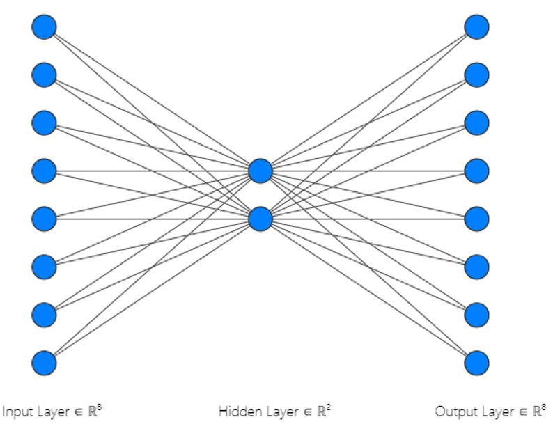

Honors Program – Thesis
Marist College – Poughkeepsie, NY

Deep Neural Network Representations for Song
Audio Matching and Recommendation

Brandon Litwin

Final Draft Received: May 16, 2019 / Accepted by Advisor: May 20, 2019

Abstract With the recent popularity of online music streaming services, com-
panies are trying to get ahead of the competition by generating accurate song
recommendations for users that are listening to their service to keep them on
the service for longer. We examine the use of autoencoders to train models
to learn which songs are similar. We found that the deep autoencoder with
multiple hidden layers produced the best results at the cost of high processing
time. Additionally, we discuss our design of a Node.js webpage that a user can
interact with and receive a recommendation of an existing song that has been
uploaded to our server.

Keywords learning representations · deep learning · autoencoders · audio ·
music · neural networks

1 Introduction

The popularity of online music streaming services such as Spotify and Apple
Music has increased rapidly in recent years. They are convenient, as a simple
monthly subscription allows consumers to access millions of songs whenever
they want. One of the most popular features of these services is their ability
to play songs by similar artists based on what the user has just listened to.
Our motivation for this project is to examine a machine learning approach
to generating song recommendations. We train autoencoders to learn how to

B. Litwin
Tel.: +1 (201) 562-6338
E-mail: brandonmlitwin@gmail.com
Honors Thesis Advisor: Pablo Rivas, Ph.D.
School of Computer Science and Mathematics
Tel.: +1 (845) 575-3000 Ext. 2086
E-mail: Pablo.Rivas@Marist.edu

2                                                                 Brandon Litwin

compress songs’ audio data to very small dimensions that we can perform low-
dimensional searches on by sound similarity. We also use the trained model to
determine which of the system’s stored song files is the most similar to a new
song that the model has never seen before.
   In this paper, we describe our methodologies finding the best autoencoder
models for comparing music files. We used three di↵erent approaches: a simple
autoencoder, an autoencoder with a sparsity constraint, and a deep-learning
autoencoder with six hidden layers. We also attempted a fourth approach: a
convolutional method, but it proved to be computationally difficult to train
on the song data. We also discuss our results and describe which of the three
approaches is the most e↵ective. Finally, we briefly explain the design of our
website that demonstrates how a user could interact with a recommendation
system like the one proposed here.

2 Background and Other Work

Typically, recommendation systems rely on usage patterns. For example, a
user can like or dislike a song and the system will use that information to
better filter its recommendations. This is known as the collaborative filtering
approach [1]. An autoencoder is a neural network model that can compress
the large amounts of data found in song files to just two dimensions to make
comparisons and visualization easier, and then it attempts to reconstruct the
data to its original dimensional space [2]; a visual explanation of a shallow au-
toencoder neural network is depicted in Fig. 1. This approach has been tested
and found to be a viable option as at least the first step in an accurate music
recommendation system [3]. Other researchers have tested a hybrid method
that uses a similar deep-learning method in combination with collaborative
filtering [4]. In the following section, we explain the design of the proposed
autoencoder.

3 Methodology

We used three di↵erent autoencoders to train on our song data. Each autoen-
coder was given twenty songs of varying genres to train on. We took vectors
of size 2.5 million, corresponding to samples taken from each song. This is
equivalent to about 57 seconds of a WAV file with 44,100 samples per second.
After each training epoch, the model’s loss was measured. We reduced the 2.5
million samples to 2 values and scaled them between 0 and 1, so that we could
graph them and get a visual representation of the similarity of songs.

3.1 Simple Autoencoder

The simple autoencoder is the most basic autoencoder with a single layer be-
tween the input and the output [2]. First, it encodes the 2.5 million samples to

DNN for Music Recommendation                                                         3

Fig. 1 Example of a shallow autoencoder neural network. This autoencoder takes an input
with eight dimensions, compresses it down to two dimensions (encoder) and then recon-
structs it back to eight dimensions (decoder).

just 2 neurons under a fully connected (Dense) layer ReLU (short for Rectified
Linear Unit) activation functions. Then, it decodes the samples back to 2.5
million using sigmoid activation functions.
    The sigmoid function [5] is given as:

                                       1             ex
                            S(x) =          x
                                                =        .                         (1)
                                     1+e            ex+1

   And the ReLU activation function [6] is given as:

                              f (x) = x+ = max(0, x).                              (2)

3.2 Sparse Autoencoder

Like the simple autoencoder, the sparse autoencoder has a single layer. The
model was the same as the simple autoencoder, with the exception that it adds
a sparsity constraint, which adds stability to the encoding process and pushes
for weight sparsity [7]. We used a regularization parameter of 10e-9. We found
that a regularizer any larger than this would result in the predictions on the
model all being very close to 0, i.e. very small weight norms.

4                                                                      Brandon Litwin

Fig. 2 Diagram of the multi-layer neural network used by the deep autoencoder.

3.3 Deep Autoencoder

The deep autoencoder adds more than one hidden layer [8]. We used three
layers, first compressing the 2.5 million samples to 32 dimensions using a linear
activation function, then 8 dimensions, then 2 dimensions. Then, the decoder
used a linear activation function to reconstruct the data back with the same
number of layers and neurons, starting with 2 dimensions, and ending with 2.5
million. The 2.5 million dimensions layer used a sigmoid function. A diagram
of the neural network used by the deep autoencoder is shown in Fig. 2.

3.4 Convolutional Autoencoder

The convolutional autoencoder that was attempted had three convolutional
layers and three pooling layers for both the encoding and decoding layers.
First, a one-dimensional convolution was applied to the 2.5 million samples,
which used the ReLU activation function, 32 filters, and a kernel size of 33.
This was followed by max pooling with a pool size of 10. Then, the result was
convolved again with 8 filters and a kernel size of 77. Then, the same pooling
function was applied, and the result was convolved a final time to 2 filters and
a kernel size of 155, and pooled once more. The decoding layers deconvolved
the filters in reverse order, starting with 2 and ending with 32. In between
each convolution, an upsampling layer of size 10 was added. Finally, the data
was deconvolved to 1 filter and a kernel size of 33 using the sigmoid activation
function.

DNN for Music Recommendation                                                    5

Fig. 3 A list of the songs that the autoencoders trained on.

  After each autoencoder model was completed, it was trained using the
Adadelta optimizer over the binary crossentropy loss function.

4 Experiments and Results

The experimental design began by selecting twenty songs of various genres
that the autoencoders would train on. We manually paired two songs from
each genre that we felt sounded similar, so that we had a reference for an
objective accuracy of the results of the autoencoders. The full song list is
shown in Fig. 3.
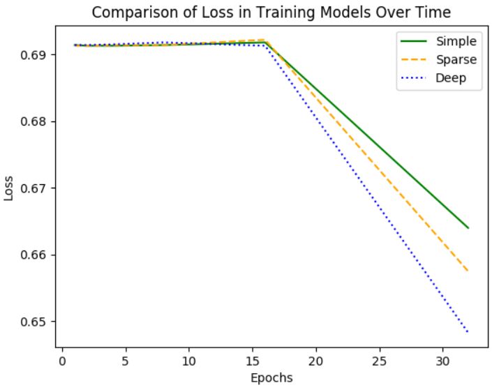
    We tested the simple and sparse autoencoders for 64 epochs, and the deep
autoencoder for 32 epochs. We found that compared to the simple autoencoder,
adding a sparsity constraint had a positive impact in reducing the loss recorded
during training. Additionally, adding more hidden layers reduced the loss the
fastest. Although the loss did not decrease for the first 16 epochs for any model,
it decreased much faster afterwards. The deep autoencoder’s loss decreased
to 0.6547 after 24 epochs and 0.6483 after 32 epochs, as shown in Fig. 4.
Comparing the plots that were generated by visualizing the encoded songs
from each training model, the simple and sparse songs are a lot more clustered
together than the deep-learning based songs, as shown in Fig. 5, Fig. 6 and
Fig. 7. The deep autoencoder more closely resembles the expected results
than the other two, with music from the same artists and music from the
same genres being closer to each other, while being further away from genres
that are much less similar to its own. For example, Let It Go and Magnolia
by Playboi Carti both produced a y-value close to 0.0. These songs are part of
the hip-hop genre and are placed far away from metal songs like Cold by At
the Gates and Take This Life by In Flames, which is expected as the songs
have distinctly di↵erent beats, melodies, instruments, and song structures. We
can argue that, without being music experts, Take This Life, with value (1.0,
1.0), and Let It Go, with value (0.0, 0.0), are polar opposites of each other.

6                                                     Brandon Litwin

Fig. 4 Comparison of loss over time between models.

Fig. 5 Simple Autoencoder Song Representations.

DNN for Music Recommendation                                                 7

Fig. 6 Sparse Autoencoder Song Representations.

Fig. 7 Deep Autoencoder Song Representations.

    The experiment on the convolutional autoencoder failed due to the training
model never reaching the second decoding layer. After decoding the data to
two dimensions with a kernel size of 155 and upsampling it once by a factor
of ten, the training model attempted to convolve the upsampled data to eight
dimensions with a kernel size of 77. After a reasonable number of minutes, the
Python script that was running the model showed no signs of progress and the
experiment was stopped.
    The computer that ran the experiments was an HP Envy x360 with an Intel
i5 processor and 8 gigabytes of RAM. Training the deep autoencoder model
takes almost 5 gigabytes of RAM. A computer with a larger amount of RAM

8                                                                 Brandon Litwin

would be able to train on more songs faster, and may be able to successfully
train our convolutional model that takes up a significant amount of memory.
    The training models ran on Keras, an open-source neural network library
for Python, which ran on top of TensorFlow. The simple, sparse, and deep
autoencoders all encoded and decoded the data with the Dense function, which
is used in sequential modeling to create a densely connected neural network
layer. This function has a parameter that can be set to the activation function
that is required. The convolutional autoencoder used the Conv1D function to
create a one-dimensional convolutional layer. It also used the MaxPooling1D
function to create pooling layers and the UpSampling1D function to upsample
the layers during decoding. We based our training models on the guide found
on Keras’s blog [9].

5 Case Study: Website For Song Matching

To test the ability of the model to be part of a production system, we deployed
it into a website. The web design consists of two Node.js webpages, a Python
script, and an SQL database. First, the user uploads a WAV file to the home
page and clicks submit. Next, the song is uploaded to the server and the Python
script is called. The Python script uses a saved learning model from a deep
autoencoder training session to create a representation of the uploaded song
in the form of two values, x and y. Using the Euclidean distance (`2 -norm),
these values are compared to each of the x and y values of the 20 songs in
the database to determine which song has values that are the closest to the
inputted song.
    The Euclidean distance formula [10] is given as:
                                    p
                          kq pk = (q p) · (q p).                             (3)

When the script is finished, the name of the recommended song is displayed
on the second webpage along with a plot of all of the songs, with a black dot
representing each song, a green circle representing the uploaded song, and a
red circle representing the song that was recommended. An example of the
resulting image that is displayed on the webpage is depicted in Fig. 8. Also,
for completeness, we include the sequence diagram for the web design (Fig. 9).
The model is successfully implemented and it only takes a moment to produce
a result.

6 Conclusions

In our research, we examined three di↵erent varieties of autoencoders that
could be used to compare the sound of songs and recommend similar sounding
songs. We determined that a deep autoencoder with multiple hidden layers
produces results that are closest to the expectation, with certain genres and
artists being grouped together. Training this model on 20 songs takes over

DNN for Music Recommendation                                                  9

Fig. 8 An example of the result image given by our website.

an hour to complete 32 epochs, while the sparse and simple models take only
10 seconds per epoch. If this model was trained on a million songs, it would
require a lot of computing resources to complete, but the finished model could
be a useful basis for music recommendation software like Spotify.

    Further research includes using recurrent neural networks to create session-
based recommendations for music streaming services. This is a potential solu-
tion to the problem of giving users accurate recommendations based on very
short sessions of data [11]. A trained autoencoder that can process a given song
quickly into a general category for comparison to other songs is a useful tool
that can be integrated into a music recommendation system. It is likely most
e↵ective to use an autoencoder along with collaborative filtering to create the
most accurate and satisfying music recommendation system for users.

10                                                                       Brandon Litwin

Fig. 9 Sequence diagram for the web design.

References

1. Van den Oord, Aaron, Sander Dieleman, and Benjamin Schrauwen. “Deep content-based
  music recommendation”. Ghent University (2013).
2. Dertat, Arden. “Applied Deep Learning: Autoencoders”. Towards Data Science (2017).
3. Liang, Dawen, Minshu Zhan, and Daniel P.W. Ellis. “Content-aware collaborative music
  recommendation using pre-trained neural networks”. Columbia University (2015).
4. Wang, Xinxi and Ye Wang. “Improving Content-based and Hybrid Music Recommenda-
  tion using Deep Learning”. National University of Singapore (2014).
5. “Sigmoid Function”. Wolfram MathWorld. Wolfram Research, Inc (2019).
6. Liu, Danqing. “ReLU - Machine Learning For Humans”. TinyMind (2017).
7. Wilkinson, Eric. “Deep Learning: Sparse Autoencoders” (2014).
8. Hubens, Nathan. “Deep inside: Autoencoders” Towards Data Science (2018).
9. Chollet, Francois. “Building Autoencoders in Keras”. The Keras Blog (2016).
10. Deza, Elena; Deza, Michel Marie. “Encyclopedia of Distances”. p. 94. Springer (2009).
11. Hidasi, Balazs et al. “Session-Based Recommendations With Recurrent Neural Net-
  works” (2016).