Gradient-Guided Dynamic Efficient Adversarial Training
←
→
Page content transcription
If your browser does not render page correctly, please read the page content below
Gradient-Guided Dynamic Efficient Adversarial Training*

                                                                         Fu Wang, Yanghao Zhang, Yanbin Zheng, Wenjie Ruan†

                                                                    Abstract                                          However, most of these solutions have been shown to ei-
                                                                                                                      ther provide “a false sense of security in defenses against
                                           Adversarial training is arguably an effective but time-                    adversarial examples” and be easily defeated by advanced
arXiv:2103.03076v1 [cs.LG] 4 Mar 2021

                                        consuming way to train robust deep neural networks that                       attacks [1]. Athalye et al. [1] demonstrate that adversarial
                                        can withstand strong adversarial attacks. As a response to                    training is an effective defense that can provide moderate or
                                        the inefficiency, we propose the Dynamic Efficient Adversar-                  even strong robustness to advanced iterative attacks.
                                        ial Training (DEAT), which gradually increases the adver-                         The basic idea of adversarial training is to utilize adver-
                                        sarial iteration during training. Moreover, we theoretically                  sarial examples to train robust DNN models. Goodfellow et
                                        reveal that the connection of the lower bound of Lipschitz                    al. [10] showed that the robustness of DNN models could
                                        constant of a given network and the magnitude of its partial                  be improved by feeding FGSM adversarial examples dur-
                                        derivative towards adversarial examples. Supported by this                    ing the training stage. Madry et al. [16] provided a uni-
                                        theoretical finding, we utilize the gradient’s magnitude to                   fied view of adversarial training and mathematically formu-
                                        quantify the effectiveness of adversarial training and deter-                 lated it as a min-max optimization problem, which provides
                                        mine the timing to adjust the training procedure. This mag-                   a principled connection between the robustness of neural
                                        nitude based strategy is computational friendly and easy to                   networks and the adversarial attacks. This indicates that a
                                        implement. It is especially suited for DEAT and can also                      qualified adversarial attack method could help train robust
                                        be transplanted into a wide range of adversarial training                     models. However, generating adversarial perturbations re-
                                        methods. Our post-investigation suggests that maintaining                     quires a significantly high computational cost. As a result,
                                        the quality of the training adversarial examples at a certain                 conducting adversarial training, especially on deep neural
                                        level is essential to achieve efficient adversarial training,                 networks, is time-consuming.
                                        which may shed some light on future studies.                                      In this paper, we aim to improve the efficiency of ad-
                                                                                                                      versarial training while maintaining its effectiveness. To
                                                                                                                      achieve this goal, we first analyze the robustness gain speed
                                        1. Introduction                                                               per epoch with different adversarial training strategies, i.e.,
                                                                                                                      PGD [16], FGSM with uniform initialization [32], and
                                           Although Deep Neural Networks (DNNs) have achieved                         FREE [22]. Although FREE adversarial training makes
                                        remarkable success in a wide range of computer version                        better use of backpropagation via its batch replay mecha-
                                        tasks, such as image classification [11, 13, 14], object detec-               nism, the visualization result shows that it is delayed by re-
                                        tion [19, 20], identity authentication [24], and autonomous                   dundant batch replays, which sometimes even cause catas-
                                        driving [9], they have been demonstrated to be vulnera-                       trophic forgetting and damage the trained model’s robust-
                                        ble to adversarial examples [3, 8, 26]. The adversarial ex-                   ness. Therefore we propose a new adversarial training strat-
                                        amples are maliciously perturbed examples that can fool a                     egy, called Dynamic Efficient Adversarial Training (DEAT).
                                        neural network and force it to output arbitrary predictions.                  DEAT begins training with one batch replay and increases
                                        There have been many works on crafting various types of                       it if the pre-defined criterion is stratified. The effectiveness
                                        adversarial examples for DNNs, e.g., [3, 16, 26–28]. In the                   of DEAT has been verified via different manual criteria. Al-
                                        meanwhile, diverse defensive strategies are also developed                    though manual approaches show considerable performance,
                                        against those adversarial attacks, including logit or feature                 they heavily depend on prior knowledge about the training
                                        squeezing [34], Jacobian regularization [4], input or feature                 task, which may hinder DEAT to be deployed on a broad
                                        denoising [29, 33], and adversarial training [10, 16, 22].                    range of datasets and model structures directly. So this leads
                                           * A Preprint. This work was done when Fu Wang was visiting Trust           to an interesting research question:
                                        AI group. Fu Wang and Yanbin Zheng were with the School of Com-
                                        puter Science and Information Security, Guilin University of Electronic          • How to efficiently quantify the effectiveness of adver-
                                        Technology. Wenjie Ruan and Yanghao Zhang were with the College of                 sarial training without extra prior knowledge?
                                        Engineering, Mathematics and Physical Sciences, University of Exeter.
                                           † Corresponding author.                                                       To answer this question, we theoretically analyze the

                                                                                                                  1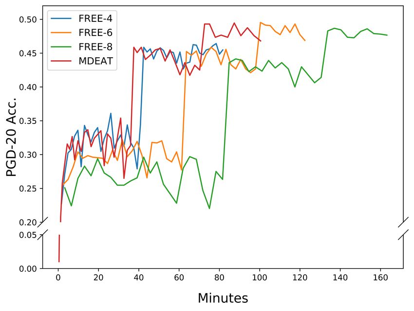
connection between the Lipschitz constant of a given net-
work and the magnitude of its partial derivative towards ad-
versarial perturbation. Our theory shows that the magnitude
of the gradient can be viewed as a reflection of the training
effect. Based on this, we propose a magnitude based ap-
proach to guide DEAT automatically, which is named M-                                             (a)
DEAT. In practice, it only takes a trivial additional compu-
tation to implement the magnitude based criterion because
the gradient has already been computed by adversary meth-
ods when crafting perturbation. Compared to other state-
of-the-art adversarial training methods, M-DEAT is highly
efficient and remains comparable or even better robust per-
formance on various strong adversarial attack tests. Besides
                                                                                                  (b)
our theoretical finding, we also explore how the magnitude
of gradient changes in different adversarial training meth-         Figure 1. Illustration of the acceleration brought by DEAT. We
ods and provide an empirical interpretation of why it mat-          plot FREE in (a) and DEAT in (b). BP is a short-hand for back-
                                                                    propagation. It can be seen that DEAT gradually increases the
ters. The takeaway here is that maintaining the quality of
                                                                    number of batch replay during training. By doing so it reduces a
adversarial examples at a certain level is more helpful to          large amount of computation for backpropagation and enables a
adversarial training than using adversarial examples gener-         more efficient training paradigm.
ated by any particular adversaries all the time.
    In summary, the key contributions of this paper lie in
three aspects:

• We analyze adversarial training methods from a perspec-           between epochs, and YOPO [36] simplifies the backpropa-
  tive on the tendency of robustness gain during training,          gation for updating training adversarial examples. A more
  which has rarely been done in previous studies.                   direct way is simply reducing the number of iteration for
                                                                    generating training adversarial examples. Like in Dynamic
• By a theoretical analysis of the connection between the           Adversarial Training [30], the number of adversarial iter-
  Lipschitz constant of a given network and its gradient to-        ation is gradually increased during training. On the same
  wards training adversarial examples, we propose an au-            direction, Friendly Adversarial Training (FAT) [38] car-
  tomatic adversarial training strategy (M-DEAT) that is            ries out PGD adversaries with an early-stop mechanism
  highly efficient and achieves the-state-of-the-art robust         to reduce the training cost. Although FGSM adversarial
  performance under various strong attacks.                         training is not effective, Wong et al. showed that FGSM
                                                                    with uniform initialization could adversarially train models
• Through comprehensive experiments, we show that the               with considerable robustness more efficiently than PGD ad-
  core mechanism of M-DEAT can directly accelerate exist-           versarial training. They also reported that cyclic learning
  ing adversarial training methods and reduce up to 60% of          rate [25] and half-precision computation [17], which are
  their time-consumption. An empirical investigation has            standard training techniques and summarized in DAWN-
  been done to interpret why our strategy works.                    Bench [5], can significantly speed up adversarial training.
                                                                    We refer the combination of these two tricks as FAST, and
2. Related Work                                                     FGSM adversarial training with uniform initialization as
                                                                    U-FGSM in the rest of this paper. Besides improvements
    Since Szegedy et al. [26] identified that modern deep           on PGD adversarial training, Shafahi et al. [22] proposed
neural networks (DNNs) are vulnerable to adversarial per-           a novel training method called FREE, which makes the
turbation, a significant number of works have been done             most use of backpass by updating the model parameters
to analyze this phenomena and defend against such a                 and adversarial perturbation simultaneously. This mech-
threat [12]. Among all these defenses, adversarial train-           anism is called batch replay, and we visualize the pro-
ing is currently the most promising method [1]. Nowa-               cess in Fig. 1(a). In parallel to efficiency, some works
days, PGD adversarial training [16] is arguably the standard        focus on enhancing the effectiveness of adversarial train-
means of adversarial training, which can withstand strong           ing. The main direction is replacing the cross-entropy loss
adversarial attacks but is extremely computationally expan-         with advanced surrogate loss functions, e.g., TRADE [37],
sive and time-consuming. Its efficiency can be improved             MMA [7], and MART [31]. Meanwhile, previous studies
from different perspectives. For example, Zheng et al. [39]         have shown that some of these loss augmentations can also
utilized the transferability of training adversarial examples       be accelerated [38].

                                                                2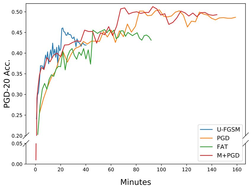
3. Preliminaries                                                      Thus, we take a closer look at the robustness gain per epoch
                                                                      during FREE adversarial training. As shown in the left col-
    Given a training set with N pairs of example and label            umn of Fig. 2, the evaluation performance of PGD-7 and U-
(xi , yi ) that are drawn i.i.d. from a distribution D, a clas-       FGSM grows linearly through the whole training process. It
sifier Fθ :PRn → Rc can be trained by minimizing a loss               is as expected that the robustness of models trained by these
               N
function i=1 L(Fθ (xi )), where n (resp. c) is the dimen-             two methods is enhanced monotonously because they only
sion of the input (resp. output) vector.                              employ a specific adversary to craft training adversarial ex-
    For the image classification task, the malevolent pertur-         amples. The training cost here, represented by the num-
bation can be added into an input example to fool the target          ber of backpropagation, are 20M and 80M for U-FGSM
classifiers [26]. As a defensive strategy, adversarial train-         and PGD-7, respectively. By contrast, the performance of
ing is formulated as the following Min-Max optimization               trained models does not increase linearly during FREE ad-
problem [15, 16]:                                                     versarial training, which is shown in the middle column
                                                                    of Fig. 2. FREE-8 spends the same amount of computa-
              min E(x,y)∼D max L(Fθ (x + δ)) ,              (1)       tional cost as PGD-7 in Fig. 2, while FREE-4 is half cheaper
             θ              δ∈B
                                                                      (40M ). We noticed that in the FREE method, the network
where the perturbation δ is generated by adversary under              is trained on clean examples in the first turn of batch replay,
condition B = {δ : kδk∞ ≤ }, which is the same `∞                   and the actual adversarial training starts at the second itera-
threat model used in [16, 22, 32].                                    tion. However, if the model is adversarially trained repeat-
   The inner maximization problem in Equ. (1) can be ap-              edly too many times on a mini-batch, catastrophic forgetting
proximated by adversarial attacks, such as FGSM [10] and              would occur and influence the training efficiency, which can
PGD [16]. The approximation calculated by FGSM can be                 be demonstrated by the unstable grown pattern of FREE-8.
written as
               δ =  · sign ∇x L(Fθ (x)) .            (2)
PGD employs FGSM with smaller step size α multiple
times and projects the perturbation back to B [16], the pro-
cedure can be described as

       δ i = δ i−1 + α · sign ∇x L(Fθ (x + δ i−1 ) .

                                                          (3)

So it can provide a better approximation to the inner maxi-
mization.
    The computational cost of adversarial training is linear
to the number of backpropagation [32]. When performing
regular PGD-i adversarial training as proposed in [16], the
adversarial version of natural training examples is generated
by a PGD adversary with i iterations. As a result, its total
number of backpropagation is proportional to (i + 1)M T ,
where M is the number of mini-batch, and T represents the
number of training epochs. By contrast, U-FGSM [32] only
uses a FGSM adversary and requires 2M T backpropaga-
tion to finish training. So from the perspective of computa-
tional cost, U-FGSM is much cheaper than PGD adversarial
training. As regarding to FREE-r adversarial training [22],           Figure 2. Illustration of the robustness gain during FAST adver-
                                                                      sarial training with PreAct-ResNet 18 on CIFAR-10. There are
which updates the model parameters and adversarial exam-
                                                                      six training strategies in this figure, and we divide them into three
ples simultaneously, it repeats training procedure r times            groups. Methods from left to right are PGD-7 & U-FGSM, FREE-
on every mini-batch and conducts rM T backpropagation                 8 & FREE-4, and DEAT-3 & DEAT-40%, respectively
to train a robust model.

4. Proposed Methodology                                               4.1. Dynamic Efficient Adversarial Training
   To further push the efficiency of adversarial training, we            These observations motivate us to introduce a new adver-
try to boost the robustness gain with as few backpropaga-             sarial training paradigm named Dynamic Efficient Adver-
tions as possible. Previous studies [2, 30] implicitly show           sarial Training (DEAT). As shown in Algorithm 1, we start
that adversarial training is a dynamic training procedure.            the training on natural examples via setting the number of

                                                                  3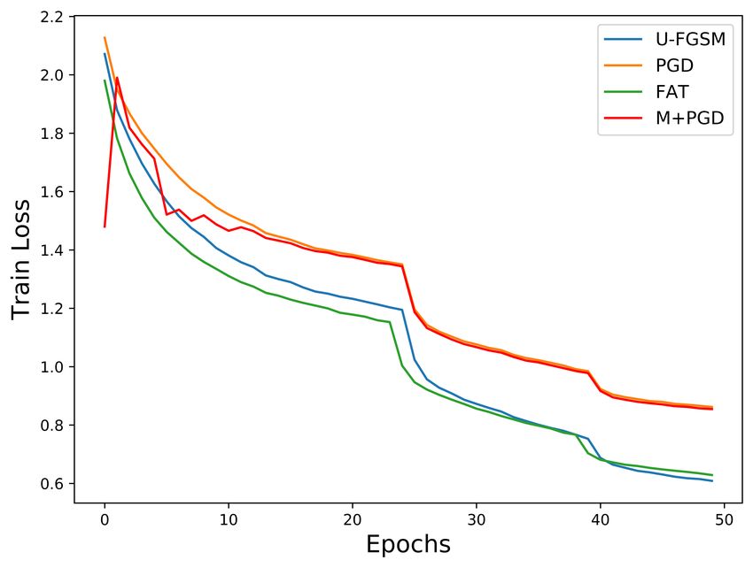
batch replay r = 1 and gradually increase it to conduct ad-                4.2. Gradient Magnitude Guided Strategy
versarial training in the later training epochs. An illustration
                                                                              To resolve the dependency on manual factors, we intro-
showing how DEAT works is presented in Fig. 1(b).
                                                                           duce a gradient-based approach to guide DEAT automati-
    A pre-defined criterion controls the timing of increas-                cally. We begin with the theoretical foundation of our ap-
ing r, and there are many possible options for the increase                proach.
criterion. Here we first discuss two simple yet effective
                                                                           Assumption 1. Let f (θ; ·) be a shorthand notation of
ways to achieve this purpose. Apparently, increasing r ev-
                                                                           L (Fθ (·)), and k · kp be the dual norm of k · kq . We assume
ery d epochs is a feasible approach. In the right column
                                                                           that f (θ; ·) satisfies the Lipschitzian smoothness condition
of Fig. 2, DEAT is first carried out at d = 3, denoted by
DEAT-3, and its computation cost is 22M that is given by                          k∇x f (θ; x) − ∇x f (θ; x̂)kp 6 lxx kx − x̂kq ,       (4)
dT (T + d)/2de. We can see that DEAT-3 only takes half
the training cost and achieves a comparable performance to                 where lxx is a positive constant, and there exists a station-
FREE-4. Although there is no adversarial robustness shown                  ary point x∗ in f (θ; ·).
at the early epoch, the DEAT-3 trained model’s robustness
                                                                               The Lipschitz condition (4) is proposed by Shaham et
shoots up significantly after training on adversarial train-
                                                                           al. [23], and Deng et al. [6] proved that the gradient-based
ing examples. Besides this naive approach, although the
                                                                           adversary can find a local maximum that supports the ex-
adversarially trained models’ robustness rises remarkably
                                                                           istence of x∗ . Then the following proposition states the
during adversarial training procedures, we observed that
                                                                           relationship between the magnitude of ∇x f (θ; x) and the
their training accuracy is only slightly above 40%. So, intu-
                                                                           Lipschitz constant lxx .
itively, 40% can be defined as a threshold to determine when
to increase r. Under this setting, denoted by DEAT-40%,                    Theorem 1. Given an adversarial example x0 = x + δ
the number of batch replay will be added one if the model’s                from the `∞ ball B . If Assumption 1 holds, then the Lips-
training accuracy is above the pre-defined threshold. As we                chitz constant lxx of current Fθ towards training example x
can see in the right column of Fig. 2, DEAT-40% achieves                   satisfies
a considerable performance with a smoother learning pro-                                      k∇x f (θ; x0 )k1
cedure compared to DEAT-3. The training cost of DEAT-                                                          6 lxx .             (5)
                                                                                                   2 |x|
40% is 25M . However, both DEAT-3 and DEAT-40% have
the same limitation, i.e., they need prior knowledge to set                Proof. Substituting x0 and the stationary point x∗
up a manual threshold, which could not be generalized di-                  into Equ. (4) gives
rectly to conduct adversarial training on different datasets
                                                                              k∇x f (θ; x0 ) − ∇x f (θ; x∗ )k1 6 lxx kx0 − x∗ k∞ .      (6)
or model architectures.
                                                                           Because x∗ is a stationary point and ∇x f (θ; x∗ ) = 0, the
                                                                           left side of Equ. (6) can be written as k∇x f (θ; x0 )k1 . The
Algorithm 1 Dynamic Efficient Adversarial Training                         right side of Equ. (6) can be simplified as
Require: Training set X, total epochs T , adversarial radius , step
    size α, the number of mini-batches M , and the number of                  lxx kx0 − x∗ k∞ = lxx kx0 − x + x − x∗ k∞
    batch replay r                                                                              6 lxx (kx0 − xk∞ + kx − x∗ k∞ )         (7)
 1: r ← 1
 2: for t = 1 to T do
                                                                                                6 lxx · (2 |x|) ,
 3:     for i = 1 to M do
                                                                           where the first inequality holds because of the trian-
 4:         Initialize perturbation δ
                                                                           gle inequality, and the last inequality holds because both
 5:         for j = 1 to r do
 6:             ∇x , ∇θ ← ∇L (Fθ (xi + δ))                                 kx0 − xk∞ and kx − x∗ k∞ are upper bounded by B that
 7:             θ ← θ − ∇θ                                                 is given by |x|, where | · | returns the size of its input.
 8:             δ ← δ + α · sign (∇x )                                     So Equ. (6) can be written as Equ. (5).
 9:             δ ← max(min(δ, ), −)
10:         end for                                                            Through Theorem 1, we can estimate a local Lipschitz
11:     end for                                                            constant lxx on a specific example x. Note that once the
12:     if meet increase criterion then                                    training set X is fixed, the 2 |x| is a constant, too. Then
13:         r ←r+1                                                         the
                                                                           P current adversarial      training effect can be estimated via
                                                                                                0
14:     end if                                                                x∈X  k∇ x f (θ; x   ) k1 or lX for short. Intuitively, a small
15: end for                                                                k∇x f (θ; x0 )k1 means that x0 is a qualified adversarial ex-
                                                                           ample that is close to a local maximum point. On the other
                                                                           hand, Theorem 1 demonstrates that k∇x f (θ; x0 )k1 can also

                                                                       4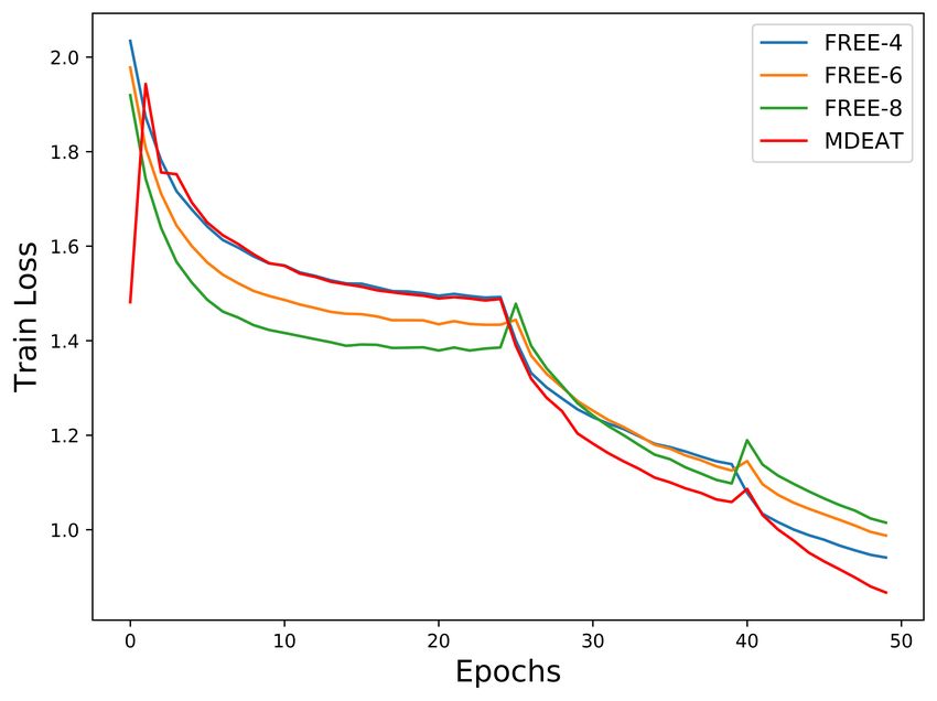
Algorithm 2 Magnitude Guided DEAT (M-DEAT)                           5.1. Under FAST Training Setting
Require: Training set X, total epochs T , adversarial radius
                                                                         We first provide our evaluation result under FAST train-
    , step size α, the number of mini-batches M , the num-
                                                                     ing setting, which utilizes the cyclic learning rate [25]
    ber of batch replay r, the evaluation of current training
                                                                     and half-precision computation [17] to speed up adversarial
    effect lX and a relax parameter γ
                                                                     training. We set the maximum of the cyclic learning rate at
 1: r ← 1
                                                                     0.1 and adopt the half-precision implementation from [32].
 2: for t = 1 to T do
                                                                     On the CIFAR-10/100 benchmarks, we compare our meth-
 3:      lX ← 0
                                                                     ods with FREE-4, FREE-8 [22], and PGD-7 adversarial
 4:      for i = 1 to M do
                                                                     training1 [16]. We report the average performance of these
 5:           Lines 4-10 in Algorithm 1     . same symbols
                                                                     methods on three random seeds. FREE methods and PGD-
 6:           lX ← lX + k∇x k1
                                                                     7 are trained with 10 epochs, which is the same setting as
 7:      end for
                                                                     in [32]. As a reminder, DEAT-3 increases the number of
 8:      if t = 1 then
                                                                     batch replay every three epochs, and DEAT-40% determines
 9:           r ←r+1
                                                                     the increase timing based on the training accuracy. DEAT-
10:      else if t = 2 then
                                                                     3 is carried out with 12 training epochs, while DEAT-40%
11:           Threshold ← γ · lX
                                                                     and M-DEAT run 11 epochs, because their first epoch are
12:      else if lX > Threshold then
                                                                     not adversarial training. All DEAT methods are evaluated
13:           Threshold ← γ · lX ; r ← r + 1
                                                                     at step size α = 10/255. We set γ = 1 for PreAct-ResNet
14:      end if
                                                                     and γ = 1.01 for Wide-ResNet.
15: end for

                                                                     CIFAR-10 As shown in Tab. 1, all DEAT methods per-
reflect the loss landscape of current Fθ , while a flat and          form properly under FAST training setting. Among three
smooth loss landscape has been identified as a key property          DEAT methods, models trained by M-DEAT show the high-
of successful adversarial training [22].                             est robustness. Because of the increasing number of batch
    From these two perspectives, we wish to maintain the             replay at the later training epochs, M-DEAT conducts more
magnitude of the gradient at a small interval via increas-           backpropagation to finish training, so it spends slightly
ing the number of batch replay. Specifically, we initial-            more on the training time. FREE-4 achieves a comparable
ize the increasing threshold in the second epoch, which is           robust performance to M-DEAT, but M-DEAT is 20% faster
also the first training epoch on adversarial examples (See           and has higher classification accuracy on the natural test
line 10 in Algorithm 2). The introduced parameter γ aims             set. The time consumption of FREE-8 almost triple those
to stabilize the training procedure. By doing so, r is only          two DEAT methods, but it only achieves a similar amount
increased when the current lX is strictly larger than in pre-        of robustness to DEAT-3. PGD-7 uses the same number of
vious epochs. In the following rounds, if lX is larger than          backpropagation as FREE-8 but performs worse.
the current threshold, DEAT will increase r by one and up-              The comparison on wide-resnet model also provides a
date the threshold. Please note that ∇x f (θ; x0 ) has already       similar result. Evaluation results on Wide-ResNet 34 ar-
been computed in ordinary adversarial training. Therefore            chitecture are presented in Tab. 2. We can see that most
M-DEAT only takes a trivial cost, i.e., compute k∇x k1 and           methods perform better than before because Wide-ResNet
update threshold, to achieve a fully automatic DEAT. In the          34 has more complex structure and more parameters than
next section, we will provide a detailed empirical study on          PreAct-ResNet 18. Although FREE-8 achieves the highest
the proposed DEAT and M-DEAT methods.                                overall robustness, its training cost is more expensive than
                                                                     others. FREE-4 also performs considerably, even it is half
5. Empirical Study                                                   cheaper than FREE-8. M-DEAT is 22% faster than FREE-4
   In this section, we report the experimental results of            with comparable robustness and achieve 97% training ef-
DEAT on CIFAR-10/100 benchmarks. All experiments are                 fect of FREE-8 with 40% time consumption. Other DEAT
built with Pytorch [18] and run on a single GeForce RTX              methods are faster than M-DEAT due to the reason that less
2080Ti. For all adversarial training methods, we set the             backpropagation has been conducted. Models trained by
batch size at 128, and use SGD optimizer with momentum               them show reasonable robustness on all tests, but their per-
0.9 and weight decay 5 · 10−4 . We use PGD-i to represent a          formance is not as good as M-DEAT. We can see that DEAT
`∞ norm PGD adversary with i iterations, while CW-i ad-              can achieve a considerable amount of robust performance.
versary optimizes the margin loss [3] via i PGD iterations.            1 The publicly available training code can be found at https://
All adversaries are carried out with step size 2/255, and the        github.com/locuslab/fast_adversarial/tree/master/
adversarial radio  is 8/255.                                        CIFAR10.

                                                                 5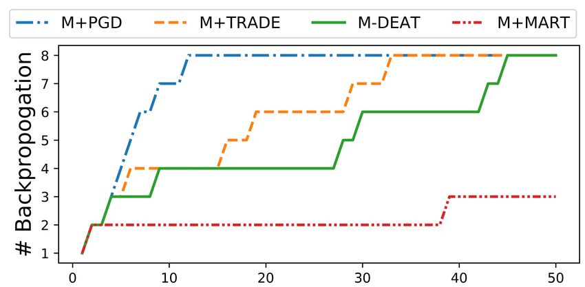
Table 1. Evaluation on CIFAR-10 with PreAct-ResNet 18. All              Table 3. Evaluation on CIFAR-100 with Wide-ResNet 34. All
methods are carried out with cyclic learning rate and half-             methods are carried out with cyclic learning rate and half-
precision.                                                              precision.
                                  Adversarial            Time                                            Adversarial            Time
  Method       Natural                                                    Method      Natural
                          FGSM     PGD-100      CW-20    (min)                                  FGSM      PGD-100      CW-20    (min)
  DEAT-3       80.09%    49.75%     42.94%      42.26%     5.8            DEAT-3      55.35%    27.24%    23.89%       22.86%    41.7
  DEAT-40%     79.52%    48.64%     42.81%      42.08%     5.6            DEAT-20%    54.42%    26.01%    22.29%       21.58%    33.4
  M-DEAT       79.88%    49.84%     43.38%      43.36%     6.0            M-DEAT      53.57%    27.19%    24.33%       23.08%    52.9
  FREE-4       78.46%    49.52%     43.97%      43.16%     7.8            FREE-4      53.50%    27.46%    24.31%       23.24%    55.8
  FREE-8       74.56%    48.60%     44.11%      42.49%    15.7            FREE-8      50.79%    27.03%    24.83%       23.04%   110.6
  PGD-7        70.90%    46.37%     43.17%      41.01%    15.1            PGD-7       43.00%    23.71%    22.38%       20.01%   109.2

Table 2. Evaluation on CIFAR-10 with Wide-ResNet 34. All meth-
ods are carried out with cyclic learning rate and half-precision.
                                                                        at 0.05 and is decayed at 25 and 40 epochs. In this exper-
                                  Adversarial            Time
  Method       Natural                                                  iment, we add FAT [38], TRADES [37], and MART [31]
                          FGSM     PGD-100      CW-20    (min)          into our comparison. FAT introduces an early stop mecha-
  DEAT-3       81.58%    50.53%     44.39%      44.43%    41.6          nism into the generation of PGD training adversarial exam-
  DEAT-40%     81.49%    51.08%     45.03%      44.49%    38.9          ples to make acceleration. Its original version is carried out
  M-DEAT       81.59%    51.29%     45.27%      45.09%    43.1
                                                                        with 5 maximum training adversarial iterations. While both
  FREE-4       80.34%    51.72%     46.17%      45.62%    55.4          original TRADES and FAT with TRADES surrogate loss,
  FREE-8       77.69%    51.45%     46.99%      46.11%   110.8
  PGD-7        72.12%    47.39%     44.80%      42.18%   109.1          denoted by F+TRADES, use 10 adversarial steps, which are
                                                                        the same settings as in [37, 38]. The same number of adver-
                                                                        sarial steps is also applied in the original MART and FAT
However, the manual criterion like DEAT-40% cannot be                   with MART surrogate loss (F+MART), which is the same
generalized properly, while M-DEAT can still perform well               settings reported in [31]. As for the hyper-parameter τ that
without any manual adjustment.                                          controls the early stop procedure in FAT, we conduct the
                                                                        original FAT, F+TRADES and F+MART at τ = 3, which
CIFAR-100 Because the classification task on CIFAR-                     enables their highest robust performance in [35]. FREE
100 is more difficult than on CIFAR-10, we test all meth-               adversarial training is conducted with three different num-
ods on Wide-ResNet. All methods are carried out under                   bers of batch replay for a comprehensive evaluation. We
the same setting except for DEAT-40%, where we man-                     only evaluate M-DEAT under this setting because those
ually change its threshold from 40% to 20%. Thus, as                    two DEAT methods cannot be deployed easily. In addition,
shown in Tab. 3, it can be observed that all baseline meth-             we also introduce our magnitude based strategy into PGD,
ods spend similar training time besides DEAT-20% and M-                 TRADE, and MART, namely M+PGD, M+TRADES, and
DEAT, which is fully automatic. M-DEAT has a similar                    M+MART. To be specific, we let the number of training
overall performance and training cost to FREE-4. Both M-                adversarial iterations start at 1 and compute the lX during
DEAT and FREE-4 outperform FREE-8, whose computa-                       training. The procedure described in lines 8–14 of Algo-
tional cost is doubled. On the other hand, although those               rithm 2 has been transplanted to control the increase of the
two DEAT methods that based on manual criterion show                    adversarial iterations2 . All magnitude based methods are
reasonable performance, they may need additional adjust-                evaluated at step size α = 10/255 and γ = 1.01 if ap-
ment to be carried out on different training settings, like             plied. As suggested in [21], each adversarial trained model
what we did on DEAT-20%.                                                is tested by a PGD-20 adversary on a validation set during
    In above experiments, we can see most methods provides              training, we save the robustest checkpoint as for the final
reasonable robustness, while PGD-7 does not fit the FAST                evaluation.
training setting and performs poorly. So we also conduct                    The experimental results are summarized in Tab. 4. We
experiments on a standard training setting, which is suitable           can see that although FREE-4 and FAT finish training
for most existing adversarial training methods.                         marginally faster than others, their classification accuracy
                                                                        on adversarial tests are substantially lower as well. Com-
5.2. Under Standard Training Setting
                                                                        pared to FREE-6, which is more efficient than FREE-8
   The experimental result under a regular training setting             and shows better robustness, M-DEAT is about 16% faster
is presented in this section. For the sake of evaluation effi-          and has higher accuracy on all evaluation tasks. PGD-
ciency, we choose the PreAct-ResNet as the default model                7 is a strong baseline under the standard training setting,
and all approaches are trained for 50 epochs with a multi-              it achieves the second robustest method when there is no
step learning rate schedule, where the learning rate starts             surrogate loss function. M+PGD outperforms PGD-7 on

                                                                    6
Table 4. Evaluation on CIFAR-10 with PreAct-ResNet 18. All
methods are carried out with multi-step learning rate and 50 train-
ing epochs.
Adversarial Time
Method Natural
FGSM PGD-100 CW-20 (min)
FREE-4 85.00% 54.47% 45.64% 46.55% 81.7
FREE-6 82.49% 54.55% 48.16% 47.42% 122.4
FREE-8 81.22% 54.05% 48.14% 47.12% 163.2
M-DEAT 84.57% 55.56% 47.81% 47.58% 100.5
PGD-7 80.07% 54.68% 49.03% 47.95% 158.8
FAT-5 84.15% 53.99% 45.49% 46.09% 91.8
M+PGD2 80.82% 55.25% 49.12% 48.13% 144.1
TRADE 79.39% 55.82% 51.48% 48.89% 456.2
Figure 3. Visualize the relationship between robustness and the
F+TRADE1 81.61% 56.31% 50.55% 48.43% 233.9
M+TRADE2 80.26% 55.69% 51.19% 48.57% 336.1 magnitude of gradient lX during U-FGSM adversarial training at
step size α = 12/255. The catastrophic overfitting occurs at
MART 75.59% 57.24% 54.23% 48.60% 147.7 epoch 23, where lX begins to shoot up.
F+MART1 83.62% 56.03% 48.88% 46.42% 234.4
M+MART2 83.64% 57.15% 48.98% 45.88% 52.1
1 Variants that are accelerated by FAT.
2 Variants that are guided by the magnitude of gradient. Table 5. Compare M-DEAT to U-FGSM under different environ-
ments. The time unit here is minute.
CIFAR10
all adversarial tests and takes 8% less time-consumption.
Set up Method Natural PGD-100 CW-20 Time
While M-DEAT is about 36% faster than PGD-7 and re-
mains a comparable robustness against the CW-20 adver- PreAct-Res. M-DEAT 79.88% 43.38% 43.36% 6.0
+ FAST1 U-FGSM 78.45% 43.86% 43.04% 5.6
sary. FAT shows highly acceleration effect on both PGD and
Wide-Res. M-DEAT 81.59% 45.27% 45.09% 43.1
TRADE. Although FAT-5 only achieves a fair robustness, + FAST U-FGSM 80.89% 45.45% 44.91% 41.3
F+TRADE’s performance is remarkable. It can seen that
PreAct-Res. M-DEAT 84.57% 47.81% 47.58% 100.5
TRADE boosts the trained model’s robustness, but also sig- + Standard2 U-FGSM 81.99% 45.77% 45.74% 40.3
nificantly increases the computational cost. F+TRADE ob-
CIFAR100
tains a comparable robustness in half of TRADE’s training
Set up Method Natural PGD-100 CW-20 Time
time. By contrast, M+TRADE is 26% faster than TRADE
and also shows a similar overall performance. Although Wide-Res. M-DEAT 53.57% 24.33% 23.08% 52.9
+ FAST U-FGSM 52.54% 24.17% 22.93% 41.6
there is no substantial improvement on the CW-20 test,
1 Training with cyclic learning rate and half-precision.
MART achieves the highest robust performance on FGSM
2 Training 50 epochs with multi-step learning rate.
and PGD-100 tests but has the lowest accuracy on natural
examples. Our M+MART reduces the time consumption of
MART almost by a factor of three, and remains a consid-
erable amount of robustness to FGSM adversary. However,
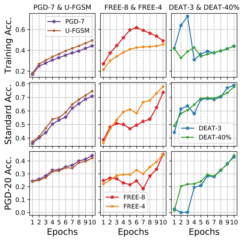
suffers from the catastrophic overfitting when its step size α
F+MART is even slower than the original MART and only
is larger than 10/255 [32]. This means the robust accuracy
achieves a similar robustness to M+MART.
of U-FGSM adversarial training with respect to a PGD ad-
versary may suddenly and drastically drop to 0% after sev-
5.3. Comparison and Collaboration with U-FGSM
eral training epochs. To address this issue, Wong et al. [32]
We report the competition between DEAT and U-FGSM randomly save a batch of training data and conduct an ad-
and demonstrate how the magnitude of gradient can help ditional PGD-5 test on the saved data. The training process
FGSM training to overcome the overfitting problem, which will be terminated if the trained model lost robustness in
is identified in [32]. The comparison is summarized the validation. We reproduce this phenomena by carrying
in Tab. 5. It is observed that the differences of robust per- out U-FGSM at α = 12/255 with a flat learning rate (0.05)
formance between U-FGSM and DEAT methods are subtle for 30 epochs and record lX during training. It can be ob-
under FAST training setting. They achieve a similar bal- served in Fig. 3 that lX surges dramatically as soon as the
ance between robustness and time consumption, while M- catastrophic overfitting occurs. By monitoring the chang-
DEAT performs better on most tests but also takes slightly ing ratio of lX , we can achieve early stopping without extra
more training time. When using the standard training set- validation. Specifically, we record lX at each epoch and be-
t
ting, U-FGSM is faster but only achieves a fair robust per- gin to calculate its changing ratio R since epoch m. Let lX
formance. Meanwhile, U-FGSM adversarial training also represent lX at epoch t, where t > m, the corresponding
7changing ratio Rt can be computed as follow:
t t−m
lX − lX
Rt = . (8)
m
We stop the training process when Rt > γ · Rt−1 , where γ
is a control parameter and plays the same role as in Algo-
rithm 2. Denoted by M+U-FGSM2 , our approach has been
evaluated at m = 2 and γ = 1.5. We report the average per-
formance of M+U-FGSM and Wong et al.’s approach on 5
random seeds in Tab. 6.
Compared with the validation based approach, we can
see that early stopping based on the changing ratio of lX is
more sensitive and maintains a stable robust performance.
The improvement on time-consumption is only trivial be-
cause this experiment is done on an advanced GPU, it
should be more visible on less powerful machines. Figure 4. lX in baseline methods under FAST training setting.
Table 6. Compare different early stopping strategies on preventing
the catastrophic overfitting. same effect and does not use multiple adversarial steps un-
Stop at Time der FAST training setting, which also explains why it works
Method Natural PGD-100
(·/30) (min) so well in Sec. 5.3. An interesting phenomena is that even
U-FGSM 75.86±1.5% 40.47±2.4% 23±2 20.2±1.5 U-FGSM only uses adversarial examples to train models,
M+U-FGSM 73.33±1.1% 41.80±0.7% 19.4±4 16.2±3.1 lX in the first epoch is still relatively higher than that in
later epochs. It seems that conduct adversarial training on
just initialized models directly would not provide a promis-
5.4. Why does lX Matter ing effectiveness.
In the last part of empirical studies, we explore why this
magnitude of gradient based strategy works. It can be seen 6. Conclusion
from previous experiments that the magnitude of gradient
lX can be deployed in different adversarial training methods To improve the efficiency of adversarial learning, we
even with loss augmentation. We then conduct an empiri- propose a Dynamic Efficient Adversarial Training called
cal investigation on how lX changes in a set of adversarial DEAT, which gradually increases the number of batch re-
training algorithms, i.e., FREE, U-FGSM, PGD-7, and M- plays based on a given criterion. Our preliminary verifica-
DEAT. They are conducted with PreAct-ResNet on CIFAR- tion shows that DEAT with manual criterion can achieve
10 under FAST training setting. Recall that lX is given by a considerable robust performance on a specific task but
P need manual adjustment to deployed on others. To re-
x∈X k∇x k1 , and a small k∇x k1 means the correspond-
ing adversarial example is close to a local minimum point. solve this limitation, we theoretically analyze the relation-
From this perspective, lX can be viewed a measurement of ship between the Lipschitz constant of a given network and
the quality of training adversarial examples. It can be ob- the magnitude of its partial derivative towards adversarial
served in Fig. 4, where illustrates that the quality of train- perturbation. We find that the magnitude of gradient can
ing adversarial examples is maintained at a certain level in be used to quantify the adversarial training effectiveness.
M-DEAT and U-FGSM. As for FREE and PGD, which em- Based on our theorem, we further design a novel criterion
ploy the same adversary at each epoch, the quality of their to enable an automatic dynamic adversarial training guided
training adversarial examples gradually decrease when the by the gradient magnitude, i.e., M-DEAT. This magnitude
trained model become more robust. This experiment sug- guided strategy does not rely on prior-knowledge or man-
gests that maintaining the quality of adversarial examples is ual criterion. More importantly, the gradient magnitude
essential to adversarial training. DEAT achieve that via in- adopted by M-DEAT is already available during the adver-
creasing the number of batch replay. Because its first train- sarial training so it does not require non-trivial extra com-
ing epoch is on natural examples with random initialized putation. The comprehensive experiments demonstrate the
perturbation, lX is high at the beginning and slumps after efficiency and effectiveness of M-DEAT. We also empiri-
adversarial examples join the training. U-FGSM has the cally show that our magnitude guided strategy can easily be
incorporated with different adversarial training methods to
2 The corresponding pseudo code is provided in supplementary material boost their training efficiency.
8An important takeaway from our studies is that main- [13] Alex Krizhevsky, Ilya Sutskever, and Geoffrey E Hinton.
taining the quality of adversarial examples at a certain level Imagenet classification with deep convolutional neural net-
is essential to achieve efficient adversarial training. In this works. In Advances in Neural Information Processing Sys-
sense, how to meaningfully measure the quality of adversar- tems (NeurIPS), 2012. 1
[14] Yann LeCun, Léon Bottou, Yoshua Bengio, and Patrick
ial examples during training would be very critical, which
Haffner. Gradient-based learning applied to document recog-
would be a promising direction that deserves further explo- nition. Proceedings of the IEEE, 86:2278–2324, 1998. 1
ration both empirically and theoretically. [15] Chunchuan Lyu, Kaizhu Huang, and Hai-Ning Liang. A uni-
fied gradient regularization family for adversarial examples.
References In International Conference on Data Mining (ICDM), 2015.
3
[1] Anish Athalye, Nicholas Carlini, and David A. Wagner. Ob- [16] Aleksander Madry, Aleksandar Makelov, Ludwig Schmidt,
fuscated gradients give a false sense of security: Circumvent- Dimitris Tsipras, and Adrian Vladu. Towards deep learning
ing defenses to adversarial examples. In 35th International models resistant to adversarial attacks. In 6th International
Conference on Machine Learning (ICML), 2018. 1, 2 Conference on Learning Representations (ICLR), 2018. 1, 2,
[2] Qi-Zhi Cai, Chang Liu, and Dawn Song. Curriculum ad-
3, 5
versarial training. In 27th International Joint Conference on [17] Paulius Micikevicius, Sharan Narang, Jonah Alben, Gre-
Artificial Intelligence (IJCAI), 2018. 3 gory F. Diamos, Erich Elsen, David Garcı́a, Boris Ginsburg,
[3] Nicholas Carlini and David Wagner. Towards evaluating the
Michael Houston, Oleksii Kuchaiev, Ganesh Venkatesh, and
robustness of neural networks. In 2017 IEEE symposium on
Hao Wu. Mixed precision training. In 6th International Con-
security and privacy (SSP), 2017. 1, 5
ference on Learning Representations (ICLR), 2018. 2, 5
[4] Alvin Chan, Yi Tay, Yew-Soon Ong, and Jie Fu. Jacobian
[18] Adam Paszke, Sam Gross, Francisco Massa, Adam Lerer,
adversarially regularized networks for robustness. In 8th In-
James Bradbury, Gregory Chanan, Trevor Killeen, Zem-
ternational Conference on Learning Representations (ICLR),
ing Lin, Natalia Gimelshein, Luca Antiga, et al. Pytorch:
2020. 1
An imperative style, high-performance deep learning li-
[5] Daniel Kang et al. Cody A. Coleman, Deepak Narayanan.
brary. In Advances in Neural Information Processing Sys-
Dawnbench: An end-to-end deep learning benchmark and
tems (NeurIPS), 2019. 5
competition. In NIPS ML Systems Workshop, 2017. 2
[19] Joseph Redmon, Santosh Kumar Divvala, Ross B. Girshick,
[6] Zhun Deng, Hangfeng He, Jiaoyang Huang, and Weijie J Su.
and Ali Farhadi. You only look once: Unified, real-time ob-
Towards understanding the dynamics of the first-order adver-
ject detection. In Conference on Computer Vision and Pat-
saries. In 37th International Conference on Machine Learn-
tern Recognition (CVPR), 2016. 1
ing (ICML), 2020. 4
[20] Shaoqing Ren, Kaiming He, Ross B. Girshick, and Jian Sun.
[7] Gavin Weiguang Ding, Yash Sharma, Kry Yik Chau Lui, and
Faster R-CNN: towards real-time object detection with re-
Ruitong Huang. MMA training: Direct input space margin
gion proposal networks. IEEE Trans. Pattern Anal. Mach.
maximization through adversarial training. In 8th Interna-
Intell., 39(6):1137–1149, 2017. 1
tional Conference on Learning Representations, ICLR, 2020.
[21] Leslie Rice, Eric Wong, and J Zico Kolter. Overfit-
2
ting in adversarially robust deep learning. arXiv preprint
[8] Yinpeng Dong, Qi-An Fu, Xiao Yang, Tianyu Pang, Hang
arXiv:2002.11569, 2020. 6
Su, Zihao Xiao, and Jun Zhu. Benchmarking adversarial ro-
[22] Ali Shafahi, Mahyar Najibi, Mohammad Amin Ghiasi,
bustness on image classification. In Conference on Computer
Zheng Xu, John Dickerson, Christoph Studer, Larry S Davis,
Vision and Pattern Recognition (CVPR), 2020. 1
Gavin Taylor, and Tom Goldstein. Adversarial training for
[9] Kevin Eykholt, Ivan Evtimov, Earlence Fernandes, Bo Li,
free! In Advances in Neural Information Processing Sys-
Amir Rahmati, Chaowei Xiao, Atul Prakash, Tadayoshi
tems (NeurIPS), 2019. 1, 2, 3, 5
Kohno, and Dawn Song. Robust physical-world attacks on
[23] Uri Shaham, Yutaro Yamada, and Sahand Negahban. Un-
deep learning visual classification. In Conference on Com-
derstanding adversarial training: Increasing local stability of
puter Vision and Pattern Recognition (CVPR), 2018. 1
supervised models through robust optimization. Neurocom-
[10] Ian J. Goodfellow, Jonathon Shlens, and Christian Szegedy.
puting, 307:195–204, 2018. 4
Explaining and harnessing adversarial examples. In 3rd In-
[24] Mahmood Sharif, Sruti Bhagavatula, Lujo Bauer, and
ternational Conference on Learning Representations (ICLR),
Michael K. Reiter. Accessorize to a crime: Real and stealthy
2015. 1, 3
attacks on state-of-the-art face recognition. In Conference on
[11] Kaiming He, Xiangyu Zhang, Shaoqing Ren, and Jian Sun.
Computer and Communications Security (CCS), 2016. 1
Deep residual learning for image recognition. In Conference
[25] Leslie N. Smith and Nicholay Topin. Super-convergence:
on Computer Vision and Pattern Recognition (CVPR), 2016.
Very fast training of neural networks using large learning
1
rates. arXiv preprint arXiv:1708.07120, 2018. 2, 5
[12] Xiaowei Huang, Daniel Kroening, Wenjie Ruan, James
[26] Christian Szegedy, Wojciech Zaremba, Ilya Sutskever, Joan
Sharp, Youcheng Sun, Emese Thamo, Min Wu, and Xinping
Bruna, Dumitru Erhan, Ian J. Goodfellow, and Rob Fer-
Yi. A survey of safety and trustworthiness of deep neural net-
gus. Intriguing properties of neural networks. In 2nd In-
works: Verification, testing, adversarial attack and defence,
ternational Conference on Learning Representations (ICLR),
and interpretability. Computer Science Review, 37:100270,
2014. 1, 2, 3
2020. 2
9[27] Florian Tramèr, Nicolas Papernot, Ian Goodfellow, Dan A. More details about our experimental results
Boneh, and Patrick McDaniel. The space of transferable ad-
versarial examples. arXiv preprint arXiv:1704.03453, 2017. As a supplement to our empirical study in the main
[28] Jonathan Uesato, Brendan O’Donoghue, Pushmeet Kohli, submission, we report the impact of the training adversar-
and Aäron van den Oord. Adversarial risk and the dangers of ial step size α in M-DEAT on the trained models under
evaluating against weak attacks. In 35th International Con- FAST training setting and provide a visualization of differ-
ference on Machine Learning (ICML), 2018. 1 ent methods’ training process under standard setting. Be-
[29] Fu Wang, Liu He, Wenfen Liu, and Yanbin Zheng. Harden
sides, we also expand the evaluation on M+U-FGSM to dif-
deep convolutional classifiers via k-means reconstruction.
ferent step sizes to test its reliability.
IEEE Access, 8:168210–168218, 2020. 1
[30] Yisen Wang, Xingjun Ma, James Bailey, Jinfeng Yi, Bowen For the purpose of reproducibility, the code of our em-
Zhou, and Quanquan Gu. On the convergence and robustness pirical study is also available in the supplementary.
of adversarial training. In 36th International Conference on
Machine Learning (ICML), 2019. 2, 3 A.1. The impact of hyper-parameters α and γ
[31] Yisen Wang, Difan Zou, Jinfeng Yi, James Bailey, Xingjun
Ma, and Quanquan Gu. Improving adversarial robustness re- We evaluate the trained models’ performance with differ-
quires revisiting misclassified examples. In 8th International ent step sizes at γ = 1.01 and γ = 1.0 respectively. Each
Conference on Learning Representations, ICLR, 2020. 2, 6 model is trained 10 epochs under the same FAST training
[32] Eric Wong, Leslie Rice, and J. Zico Kolter. Fast is better than setting, and each combination of α and γ was tested on 5
free: Revisiting adversarial training. In 8th International random seeds. To highlight the relationship between mod-
Conference on Learning Representations (ICLR), 2020. 1, els’ robustness and the corresponding training cost, which
3, 5, 7 is denoted by the number of backpropagation (#BP), we use
[33] Cihang Xie, Yuxin Wu, Laurens van der Maaten, Alan L.
Yuille, and Kaiming He. Feature denoising for improving
PGD-20 error that is computed as one minus model’s classi-
adversarial robustness. In Conference on Computer Vision fication accuracy on PGD-20 adversarial examples. The re-
and Pattern Recognition (CVPR), 2019. 1 sult has been summarized in Fig. 5. This experiment shows
[34] Weilin Xu, David Evans, and Yanjun Qi. Feature squeezing: that M-DEAT can be carried out at a large range of α. Al-
Detecting adversarial examples in deep neural networks. In though M-DEAT achieves a slightly better robust perfor-
25th Annual Network and Distributed System Security Sym- mance when carrying out at a large step size, like 14/255,
posium (NDSS), 2018. 1 the corresponding training cost is much higher than that at
[35] Runtian Zhai, Chen Dan, Di He, Huan Zhang, Boqing lower step size. Therefore, as we mentioned in the main
Gong, Pradeep Ravikumar, Cho-Jui Hsieh, and Liwei Wang.
submission that all DEAT methods are evaluated at step
MACER: attack-free and scalable robust training via maxi-
mizing certified radius. In 8th International Conference on
size α = 10/255. We set γ = 1 for PreAct-ResNet and
Learning Representations (ICLR), 2020. 6 γ = 1.01 for Wide-ResNet when using the FAST training
[36] Dinghuai Zhang, Tianyuan Zhang, Yiping Lu, Zhanxing setting, while all magnitude based methods are carried out
Zhu, and Bin Dong. You only propagate once: Accelerat- at γ = 1.01 under standard training setting.
ing adversarial training via maximal principle. In Advances
in Neural Information Processing Systems (NeurIPS), 2019. A.2. Visualize the training process under standard
2 training
[37] Hongyang Zhang, Yaodong Yu, Jiantao Jiao, Eric P. Xing,
Laurent El Ghaoui, and Michael I. Jordan. Theoreti- In the main submission, we introduce the magnitude of
cally principled trade-off between robustness and accuracy. trained model’s partial derivative towards adversarial exam-
In 36th International Conference on Machine Learning ples to guide our DEAT and existing adversarial methods
(ICML), 2019. 2, 6 under a standard training setting with the PreAct-ResNet ar-
[38] Jingfeng Zhang, Xilie Xu, Bo Han, Gang Niu, Lizhen chitecture. A complete version of M-DEAT’s pseudo code
Cui, Masashi Sugiyama, and Mohan S. Kankanhalli. At- is shown in Algorithm 3, while M+PGD, M+TRADE, and
tacks which do not kill training make adversarial learning
M+MART can be descried by Algorithm 4 via changing
stronger. In 37th International Conference on Machine
Learning (ICML), 2020. 2, 6
loss functions. Note that we adjust the step size α∗ per
[39] Haizhong Zheng, Ziqi Zhang, Juncheng Gu, Honglak Lee, epoch based on the number of adversarial steps r and the
and Atul Prakash. Efficient adversarial training with trans- adversarial radio to make sure that α∗ · r ≥ for the
ferable adversarial examples. In Conference on Computer methods that are guided by the gradient magnitude. All
Vision and Pattern Recognition (CVPR), 2020. 2 models were trained 50 epochs with a multi-step learning
rate schedule, where the learning rate starts at 0.05 and is
decayed at 25 and 40 epochs. To better present our experi-
ment under this scenario, we visualize the training process
of all methods from two perspectives to show the how mod-
els gain their robustness toward the PGD-20 adversary and
10to the loss change of M+PGD and PGD are highly coinci-
dent at the late training stage, because M+PGD conducted
the same adversarial steps as in PGD during this period.
The result of TRADE related adversarial training methods
is summarized in Fig. 7(c). M+TRADE performs similar
to F+TRADE at the early training stage, but it is less effi-
cient than F+TRADE because of the increased adversarial
iterations. As shown in Fig. 8(c), the lines corresponding to
the loss change of M+TRADE and TRADE are also coin-
cident at the late training stage. MART adversarial training
methods are summarized in Fig. 7(d) and Fig. 8(d). We
can observe from Fig. 8(d) that the curves of MART and
M+MART fluctuate similarly during the whole training pro-
cess, while the loss of F+MART decreased steadily.
To sum up, the approaches that adopts the magnitude
guided strategies can reduce the adversarial steps at the
early training stage to accelerate the training process. Fig. 6
visualizes the number of backpropagation w.r.t epochs,
where our magnitude-guided strategy shows adaptive capa-
bility when accelerating different methods.
Figure 5. Visualize the impact of α and γ. #BP is a short-hand
for the number of backpropagation. PGD-20 error is computed as
one minus model’s classification accuracy of PGD-20 adversarial Figure 6. The number of backpropagation w.r.t epochs.
examples.
A.3. Evaluate M+U-FGSM with different step sizes
how their training loss are decreased during the adversarial
training. In section, we evaluate M+U-FGSM at step size α ∈
{12, 14, 16, 18} to test its reliability on preventing the catas-
As shown in Fig. 7(a) that the models’ robustness surges
trophic overfitting. M+U-FGSM achieves early stopping
after each learning rate decays. Because M-DEAT only
via monitoring the changing ratio of the magnitude of gra-
does a few batch replays at the early training stage, it fin-
dient, which is shown in lines 9–14 in Algorithm 5. The ex-
ishes training earlier than FREE-6 and FREE-8, and the
perimental result is summarized in Tab. 7, where we can see
model trained by it shows a comparable robust performance
that M+U-FGSM provides a reasonable performance under
to FREE methods. FREE-4 uses the least training time but
different settings and is as reliable as the validation based
shows a less competitive robust performance at the final
U-FGSM to avoid overfitting. It can also be observed that
training stage. The corresponding loss change during train-
a larger step size does not improve the models’ robustness
ing is plotted in Fig. 8(a). The training process of PGD-7,
and may lead to an earlier occurrence of overfitting.
FAT, U-FGSM, and M+PGD is summarized in Fig. 7(b).
We observe that although U-FGSM and FAT are faster
than PGD and M+PGD, their robust performance is lower.
M+PGD finish training about 10 minutes earlier than PGD
and achieve a higher robust performance after the second
learning rate decay. In practice, we set an upper bound on
the number of adversarial step for M+PGD, which is the
same as in PGD. So the acceleration of M+PGD comes
from the reduced adversarial steps at early training stage.
It can be seen from Fig. 8(b) that the lines corresponding
11(a) (b)
(c) (d)
Figure 7. An illustration about how adversarially trained models gain robustness. We employ a PGD-20 adversary to test a model on the
the first 1280 examples of the CIFAR-10 test set after each training epoch. All methods in this part have been divided into four groups.
M-DEAT and three FREE methods are plotted in (a), M+PGD, U-FGSM, FAT, and PGD are plotted in (b). TRADES related methods and
MART related methods are shown in (c) and (d) respectively.
Table 7. Compare magnitude guided early stopping (M+U-FGSM)
to validation based early stopping (U-FGSM) on preventing the
catastrophic overfitting at different step sizes over 5 random seeds.
Stop at Time
α Natural PGD-100
(·/30) (min)
M+U-FGSM
12 73.33±1.1% 41.80±0.7% 19.4±4 16.2±3.1
14 72.25±1.0% 41.07±0.8% 17.8±2 14.5±1.6
16 70.64±1.5% 40.64±0.6% 15.4±1 12.6±0.5
18 71.51±1.9% 40.90±0.9% 15.8±2 12.6±1.4
U-FGSM
12 75.86±1.5% 40.47±2.4% 23±2 20.2±1.5
14 72.36±1.0% 40.77±1.1% 17.4±2 15.9±1.7
16 72.37±0.7% 40.98±0.5% 15.6±1 13.6±0.7
18 72.92±0.9% 39.35±4.2% 16.6±2 14.2±1.3
12(a) (b)
(c) (d)
Figure 8. An illustration of the training loss of different adversarial training methods. All methods in this part have been divided into
four groups. M-DEAT and three FREE methods are plotted in (a), M+PGD, U-FGSM, FAT, and PGD are plotted in (b). TRADES related
methods and MART related methods are shown in (c) and (d) respectively.
13Algorithm 3 Magnitude Guided DEAT (M-DEAT)
Require: Training set X, total epochs T , adversarial radius , step
size α, the number of mini-batches M , the number of batch
replay r, the evaluation of current training effect lX and a re-
lax parameter γ
1: r ← 1
2: for t = 1 to T do
3: lX ← 0
4: for i = 1 to M do
5: Initialize perturbation δ
6: for j = 1 to r do
7: ∇x , ∇θ ← ∇L (Fθ (xi + δ))
8: θ ← θ − ∇θ
9: δ ← δ + α · sign (∇x )
10: δ ← max(min(δ, ), −)
11: end for
12: lX ← lX + k∇x k1
13: end for
14: if t = 1 then Algorithm 5 M+U-FGSM
15: r ←r+1
Require: Training set X, total epochs T , adversarial radius , step
16: else if t = 2 then
size α and number of minibatches M , Compute the changing
17: Threshold ← γ · lX
ratio R since epoch m, and a relax parameter γ.
18: else if lX > Threshold then
1: for t = 1 . . . T do
19: Threshold ← γ · lX ; r ← r + 1
2: lX ← 0
20: end if
3: for i = 1 . . . M do
21: end for
4: δ = U(−, )
5: δ = δ + α · sign (∇δ Lce (xi + δ, yi , k))
6: δ = max(min(δ, ), −)
7: θ = θ − ∇θ Lce (Fθ (xi + δ) , yi )
Algorithm 4 Magnitude Guided PGD (M+PGD)
8: end for
Require: Training set X, total epochs T , adversarial radius , step 9: if t > m then
size α, the number of mini-batches M , the number of PGD lt −lt−m
10: Rt = X mX
steps N , the evaluation of current training effect lX and a relax
11: if Rt > γ · Rt−1 then
parameter γ
12: Stop training
1: r ← 1
13: end if
2: for t = 1 to T do
14: end if
3: α∗ ← Adjustment(r, , α)
15: end for
4: lX ← 0
5: for i = 1 to M do
6: Initialize perturbation δ
7: for j = 1 to N do
8: ∇x ← ∇L (Fθ (xi + δ))
9: δ ← δ + α∗ · sign (∇x )
10: δ ← max(min(δ, ), −)
11: end for
12: lX ← lX + k∇x k1
13: θ ← θ − ∇θ L (Fθ (xi + δ))
14: end for
15: if t = 1 then
16: r ←r+1
17: else if t = 2 then
18: Threshold ← γ · lX
19: else if lX > Threshold then
20: Threshold ← γ · lX ; r ← r + 1
21: end if
22: end for
14You can also read