Harvesting Large-Scale Weakly-Tagged Image Databases from the Web
←
→
Page content transcription
If your browser does not render page correctly, please read the page content below
Harvesting Large-Scale Weakly-Tagged Image Databases from the Web

                            Jianping Fan1 , Yi Shen1 , Ning Zhou1 , Yuli Gao2
                     1
                       Department of Computer Science, UNC-Charlotte, NC28223, USA
              2
                Multimedia Interaction and Understanding, HP Labs, Palo Alto, CA94304, USA

                        Abstract                                   new algorithm for harvesting image databases from the web
                                                                   by combining text, meta-data and visual information. All
To leverage large-scale weakly-tagged images for computer          these existing techniques have made a hidden assumption,
vision tasks (such as object detection and scene recogni-          e.g., image semantics have an explicit correspondence with
tion), a novel cross-modal tag cleansing and junk image            the associated texts or nearby texts. Unfortunately, such an
filtering algorithm is developed for cleansing the weakly-         assumption may not always be true.
tagged images and their social tags (i.e., removing irrele-            Collaborative image tagging system, such as Flickr [3],
vant images and finding the most relevant tags for each im-        is now a popular way to obtain large set of labeled images
age) by integrating both the visual similarity contexts be-        easily by relying on the collaborative effort of a large pop-
tween the images and the semantic similarity contexts be-          ulation of Internet users. In a collaborative image tagging
tween their tags. Our algorithm can address the issues of          system, people can tag the images according to their social
spams, polysemes and synonyms more effectively and de-             or cultural backgrounds, personal expertise and perception.
termine the relevance between the images and their social          We call the collaboratively-tagged images as weakly-tagged
tags more precisely, thus it can allow us to create large          images because their social tags may not have exact cor-
amounts of training images with more reliable labels by har-       respondences with the underlying image semantics. With
vesting from large-scale weakly-tagged images, which can           the exponential growth of the weakly-tagged images, it is
further be used to achieve more effective classifier training      very attractive to develop new algorithms that can lever-
for many computer vision tasks.                                    age large-scale weakly-tagged images for computer vision
                                                                   tasks (such as learning the classifiers for object detection
1. Introduction                                                    and scene recognition). Without controlling the word vo-
                                                                   cabulary, many text terms for image tagging may be syn-
For many computer vision tasks, such as object detection           onyms or polysemes or even spams. The appearances of
and scene recognition, machine learning techniques are usu-        synonyms, polysemes and spams may either return incom-
ally involved to learn the classifiers from a set of labeled       plete sets of the relevant images or result in large amounts
training images [1]. The size of the labeled training images       of ambiguous images or even junk images. Thus it is not
must be large-scale due to: (1) the number of object classes       a trivial task to leverage large-scale weakly-tagged images
and scenes of interest could be very large; (2) the learning       for computer vision tasks.
complexity for some object classes and scenes could be very            In this paper, we focus on collecting large-scale weakly-
high because of visual ambiguity; and (3) a small number           tagged images from collaborative image tagging systems
of labeled training images are incomplete or insufficient to       such as Flickr by addressing the following crucial issues:
interpret the diverse visual properties of large amounts of            (a) Synonymous Tags: Different people may use dif-
unseen test images. However, hiring professionals to label         ferent tags, which have the same or close meanings (syn-
large amounts of training images is cost-sensitive and poses       onyms), to tag their images. For example, car, auto, and au-
a key limitation for the practical use of some advanced com-       tomobile are a set of synonyms. The synonyms may result
puter vision techniques. On the other hand, large-scale dig-       in incomplete returns of the relevant images in the image
ital images and their associated text terms are available on       crawling process, and most tag clustering algorithms can-
the Internet, thus it is very attractive to leverage large-scale   not incorporate the visual similarities between the relevant
online images for computer vision tasks [2].                       images to deal with the issue of synonyms more effectively.
    Some pioneering works have been done to leverage In-               (b) Polysemous Tags: Collaborative image tagging is
ternet images for computer vision tasks [2, 4-8]. Fergus et        an ambiguous process. Without controlling the vocabulary,
al. [4] and Li et al. [6] dealt with the precision problem by      different people may apply the same tag in different ways
re-ranking the images which are downloaded from an image           (i.e., the same tag may have different meanings under dif-
search engine. Recently, Schroff et al. [7] have developed a       ferent contexts), which may result in large amounts of am-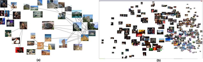
biguous images. For example, the text term “bank” can be               The occurrence frequency for each content-relevant tag
used to tag “bank office”, “river bank” and “cloud bank”.          and each event-relevant tag is counted automatically by us-
Word sense disambiguation is one potential solution for ad-        ing the number of relevant images. The misspelling tags
dressing this ambiguity issue, but it cannot incorporate the       may have low frequencies (i.e., different people may make
visual properties of the relevant images to deal with the is-      different typing mistakes), thus it is easy for us to correct
sue of polysemes more effectively [9-10].                          such the misspelling tags and their images are added into
    (c) Spam Tags: Spam tags, which are used to drive traf-        the relevant tags automatically. Two tags, which are used
fic to certain images for fun or profit, are done by inserting     for tagging the same image, are considered to co-occur once
the text terms that are more related to popular query terms        without considering their order. A co-occurrence matrix is
rather than the text terms related to the actual image con-        obtained by counting the frequencies of such pairwise tag
tent. Spam tags are problematic because the junk images            co-occurrences.
may mislead the underlying machine learning tools for clas-            The content-relevant tags and the event-relevant tags are
sifier training. Junk image filtering is an attractive direction   further partitioned into two categories according to their
for dealing with the issue of spam tags, but it is worth noting    interestingness scores: interesting tags and uninteresting
that the scenario for junk image filtering in a collaborative      tags. In this paper, multiple information sources have been
image tagging space is significantly different.                    exploited for determining the interesting tags more accu-
    In this paper, a novel cross-modal tag cleansing and           rately. For a given tag C, its interestingness score ω(C)
junk image filtering algorithm is developed by integrat-           depends on: (1) its occurrence frequency t(C) (e.g., higher
ing both the visual properties of the weakly-tagged images         occurrence frequency corresponds to higher interestingness
and their social tags to deal with the issues of spams, pol-       score); and (2) its co-occurrence frequency ϑ(C) with any
ysemes and synonyms more effectively, so that we can cre-          other tag in the vocabulary (e.g., higher co-occurrence fre-
ate large amounts of training images with more reliable la-        quency corresponds to higher interestingness score). The
bels for computer vision tasks by harvesting from large-           occurrence frequency t(C) for a given tag C is equal to the
scale weakly-tagged images. The paper is organized as fol-         number of images that are tagged by the given tag C. The
lows. In section 2, an automatic algorithm is introduced for       co-occurrence frequency ϑ(C) for the given tag C is equal
image topic extraction. In section 3, a mixture-of-kernels         to the number of images that are tagged jointly by the given
algorithm is introduced for image similarity characteriza-         tag C and any other tag in the vocabulary.
tion. In section 4, a spam tag detection technique is intro-           The interestingness score ω(C) for a given tag C is de-
duced for junk image filtering. In section 5, a cross-modal        fined as:
tag cleansing algorithm is introduced for addressing the is-                            p                           p
                                                                   ω(C) = ξ·log(t(C)+     t2 (C) + 1)+ζ·log(ϑ(C)+      ϑ2 (C) + 1)
sues of synonyms and polysemes. The algorithm evaluation                                                                      (1)
results are given in section 6. We conclude this paper at           where ξ and ζ are the weighting factors, ξ +ζ = 1.
section 7.                                                             All the interesting tags, which have large values of Ω(·)
                                                                   (i.e., top 5000 tags in our current experiments), are treated
2. Image Topic Extraction                                          as image topics. In this work, only the interesting tags,
                                                                   which are used to interpret the most popular real-world ob-
Each image in a collaborative tagging system is associated         ject classes and scenes or events, are treated as the image
with the image holder’s taggings of the underlying image           topics. It is worth noting that one single weakly-tagged im-
content and other users’ taggings or comments. It is worth         age may be assigned into multiple image topics when the
noting that entity extraction can be done more effectively in      relevant tags are used for tagging the image jointly. Collect-
a collaborative image tagging space. In this paper, we first       ing large-scale training images for the most popular real-
focus on extracting the social tags which are strongly related     world object classes and scenes or events and learning their
to the most popular real-world objects and scenes or events.       classifiers more accurately are crucial for many computer
The social tags, which are related to image capture time and       vision tasks.
place, are also very attractive, but they are beyond the scope
of this paper. Thus the image tags are first partitioned into      3. Image Similarity Characterization
two categories: noun phrases versus verb phrases. The noun
phrases are further partitioned into two categories automat-       To achieve more sufficient characterization of various visual
ically: content-relevant tags (i.e., tags that are relevant to     properties of the images, both global and local visual fea-
image objects and scenes) and content-irrelevant tags. The         tures are extracted for image content representation. In our
verb phrases are further partitioned into two categories au-       current experiments, the following visual features are ex-
tomatically: event-relevant tags (i.e., tags that are relevant     tracted: (1) 36-bin RGB color histogram to characterize the
to image events) and event-irrelevant tags.                        global color distributions of the images; (2) 48-dimensional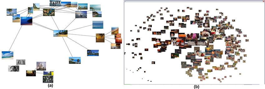
texture features from Gabor filter banks to characterize the     4. Spam Tag Detection
global visual properties (i.e., global structures) of the im-
ages; and (3) a number of interest points and their SIFT         Some popular image topics in the vocabulary may consist of
(scale invariant feature transform) features to characterize     large amounts of junk images because of spam tagging, and
the local visual properties of the underlying salient image      incorporating the junk images for classifier training may se-
components.                                                      riously mislead the underlying machine learning tools. Ob-
                                                                 viously, the junk images, which are induced by spam tag-
   By using high-dimensional visual features (color his-         ging, may make a significant difference on their visual prop-
togram, wavelet textures, and SIFT features) for image con-      erties with the relevant images. Thus the junk images can
tent representation, it is able for us to characterize various   be filtered out effectively by performing visual-based image
visual properties of the images more sufficiently. On the        clustering and relevance analysis.
other hand, the statistical properties of the images in the
high-dimensional feature space may be heterogeneous be-
cause different feature subsets are used to characterize dif-    4.1    Image Clustering
ferent visual properties of the images, thus the statistical
                                                                 A K-way min-max cut algorithm is developed to achieve
properties of the images in the high-dimensional feature
                                                                 more effective image clustering, where the cumulative inter-
space may be heterogeneous and sparse. Therefore, it is
                                                                 cluster visual similarity contexts are minimized while the
hard to use only one single type of kernel to characterize
                                                                 cumulative intra-cluster visual similarity contexts (summa-
the diverse visual similarity contexts between the images
                                                                 tion of pairwise image similarity contexts within a cluster)
precisely.
                                                                 are maximized. These two criteria can be satisfied simulta-
    Based on these observations, the high-dimensional vi-        neously with a simple K-way min-max cut function [11].
sual features are first partitioned into multiple feature sub-      For a given image topic C, a graph is first constructed for
sets and each feature subset is used to characterize one cer-    organizing all its weakly-tagged images according to their
tain type of visual properties of the images, thus the un-       visual similarity contexts [11-12], where each node on the
derlying visual similarity contexts between the images are       graph is one weakly-tagged image for the given image topic
more homogeneous and can be approximated more pre-               C and an edge between two nodes is used to characterize
cisely by using one particular type of kernel. For each fea-     the visual similarity contexts between two weakly-tagged
ture subset, a suitable base kernel is designed for image sim-   images, κ(·, ·).
ilarity characterization. Because different base image ker-         All the weakly-tagged images for the given image topic
nels may play different roles on characterizing the diverse      C are partitioned into K clusters automatically by minimiz-
visual similarity contexts between the images, the optimal       ing the following objective function:
kernel for diverse image similarity context characterization
                                                                                                   K
                                                                               (                                       )
can be approximated more accurately by using a linear com-                                         X s(Gi , G/Gi )
bination of these base image kernels with different impor-                min Ψ(C, K, β) =                                  (3)
                                                                                                   i=1
                                                                                                         s(Gi , Gi )
tance.
    For a given image topic Cj in the vocabulary, differ-        where G = {Gi |i = 1, · · · , K} is used to represent K im-
ent base image kernels may play different roles on charac-       age clusters, G/Gi is used to represent other K − 1 image
terizing the diverse visual similarity relationships between     clusters in G except Gi , K is the total number of image
the images. Thus the diverse visual similarity contexts be-      clusters, β is the set of the optimal kernel weights. The cu-
tween the images are characterized more precisely by using       mulative inter-cluster visual similarity context s(Gi , G/Gi )
a mixture-of-kernels [13-14]:                                    is defined as:
                                                                                                X X
                                                                             s(Gi , G/Gi ) =                κ(u, v)        (4)
                    τ                     τ
                    X                     X                                                     u∈Gi v∈G/Gi
        κ(x, y) =         βl κl (x, y),         βl = 1    (2)
                    l=1                   l=1                    The cumulative intra-cluster visual similarity context
                                                                 s(Gi , Gi ) is defined as:
where τ is the number of feature subsets (i.e., the number                                      X X
of base image kernels), βl ≥ 0 is the importance factor                         s(Gi , Gi ) =               κ(u, v)         (5)
                                                                                                u∈Gi v∈Gi
for the lth base image kernel κl (x, y). Combining multiple
base kernels can allow us to achieve more precise charac-
                                                                    We further define X = [X1 , · · · , Xl , · · · , Xk ] as the
terization of the diverse visual similarity contexts between
                                                                 cluster indicators, and its component Xl is a binary indi-
the weakly-tagged images.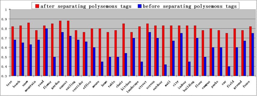
Figure 1: Image clustering for the image topic “beach”: (a) cluster correlation network; (b) filtered junk images.
cator for the appearance of the lth cluster Gl , The objective function for kernel weight determination
is to maximize the inter-cluster separability and the intra-
1, u ∈ Gl cluster compactness. For one specific cluster Gl , its inter-
Xl (u) = (6) cluster separability µ(Gl ) and its intra-cluster compactness
0, otherwise
σ(Gl ) are defined as:
W is defined as an n×n symmetrical matrix (i.e., n is the µ(Gl ) = XlT (D − W )Xl , σ(Gl ) = XlT W Xl (12)
total number of web images), and its component is defined
as: For one specific cluster Gl , we can refine its cumulative
Wu,v = κ(u, v) (7) intra-cluster pairwise image similarity contexts s(Gl , Gl ) as
W (Gl ):
D is defined as an n × n diagonal matrix, and its diagonal
τ
components are defined as: X X X
W (Gl ) = κ(u, v) = βi ωi (Gl ) (13)
n
X u∈Gl v∈Gl i=1
Du,u = Wu,v (8)
τ
v=1 X
D(Gl ) − W (Gl ) = βi [i (Gl ) − ωi (Gl )] (14)
For the given image topic C, an optimal partition of its i=1
weakly-tagged images (i.e., image clustering) is achieved where ωi (Gl ) and i (Gl ) are defined as:
by:
X X nl
X
K ωi (Gl ) = κi (u, v), i (Gl ) = ωi (Gl ) (15)
( )
X XlT (D − W )Xl
min Ψ(C, K, β) = (9) u∈Gl v∈Gl v=1
l=1
XlT W Xl
The optimal weights β ~ = [β1 , · · ·, βτ ] for kernel com-
−
→ 1 1 −
→ D2
1
Xl bination are determined automatically by maximizing the
Let W = D− 2 W D− 2 , and Xl = 1 , the objective
kD 2 Xl k inter-cluster separability and the intra-cluster compactness:
function for our K-way min-max cut algorithm can further
be refined as: ( K
)
max 1 X σ(Gl )
~ (16)
K β K µ(Gl )
( )
X 1 l=1
min Ψ(C, K, β) = −
→T − → − → −K (10)
l=1 Xl · W · Xl
Pτ
subject to: i=1 βi = 1, ∀i : βi ≥ 0
The optimal kernel weights β~ = [β1 , · · ·, βτ ] are de-
subject to:
termined automatically by solving the following quadratic
−
→T − → −
→T − → − → programming problem:
Xl · Xl = I, Xl · W · Xl > 0, l ∈ [1, · · · , K]
K
( ! )
The optimal solution for Eq. (10) is finally achieved by min 1 ~T X T ~
~ β Ω(Gl )Ω(Gl ) β (17)
solving multiple eigenvalue equations: β 2
l=1
−
→ − → −
→ Pτ
W · Xl = λ l Xl , l ∈ [1, · · · , K] (11) subject to: i=1 βi = 1, ∀i : βi ≥ 0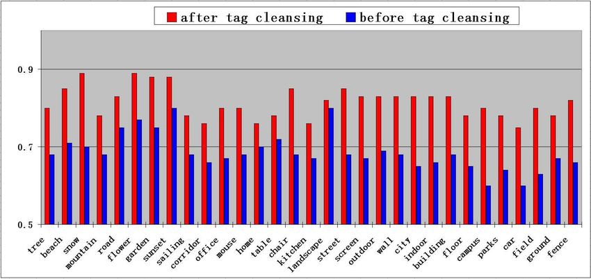
Figure 2: Image clustering for the image topic “rock”: (a) cluster correlation network; (b) filtered junk images.

   Ω(Gl ) is defined as:                                             are used to indicate the co-occurrence probabilities for the
                                                                     images x and y with the image topic C.
                                  ω(Gl )                                 In order to leverage the inter-cluster correlations for
                  Ω(Gl ) =                                   (18)
                              (Gl ) − ω(Gl )                        achieving more effective relevance re-ranking, a random
                                                                     walk process is performed for automatic relevance score re-
    In summary, our K-way min-max cut algorithm takes the
                                                                     finement [15]. For a given image topic C, our image cluster-
following steps iteratively for image clustering and kernel
                                                                     ing algorithm can automatically determine a cluster corre-
weight determination: (1) β is set equally for all these fea-
                                                                     lation network (i.e., K image clusters and their inter-cluster
ture subsets at the first run of iterations. (2) Given the initial
                                                                     correlations) as shown in Fig. 1(a) and Fig. 2(a). We use
values of kernel weights, our K-way min-max cut algorithm
                                                                     ρl (Gi ) to denote the relevance score for the ith image clus-
is performed to partition the weakly-tagged images into K
                                                                     ter Gi at the lth iteration. The relevance scores for all these
clusters according to their pairwise visual similarity con-
                                                                     K image clusters at the lth iteration will form a column vec-
texts. (3) Given an initial partition of the weakly-tagged               −−−→
images, our kernel weight determination algorithm is per-            tor ρ(Gi ) ≡ [ρl (Gi )]K×1 . We further define Φ as an K × K
formed to estimate more suitable kernel weights, so that             transition matrix, its element φGi ,Gj is used to define the
more precise characterization of the diverse visual similar-         probability of the transition from the image cluster Gi to its
ity contexts between the images can be achieved. (4) Go to           inter-related image cluster Gj . φGi ,Gj is defined as:
step 2 and continue the loop iteratively until β is convergent.
As shown in Fig. 1(a) and Fig. 2(a), our image cluster-                                               s(Gi , Gj )
                                                                                      φGi ,Gj = P                               (20)
ing algorithm can achieve a good partition of large amounts                                          Gh ∈C s(Gi , Gh )
of weakly-tagged images and determine their global distri-
butions and inter-cluster correlations effectively. Unfortu-         where s(Gi , Gj ) is the inter-cluster visual similarity context
nately, such image clustering process cannot directly iden-          between two image clusters Gi and Gj as defined in Eq. (4).
tify the clusters for the junk images.                                  The random walk process is then formulated as:
                                                                                     X
                                                                      ρl (Gi ) = θ          ρl−1 (Gj )φGi ,Gj + (1 − θ)ρ(C, Gi ) (21)
4.2    Relevance Re-Ranking                                                          j∈Ωj
For different users, their motivations for spam tagging are
significantly different and their images for spam tagging            where Ωj is the first-order nearest neighbors of the image
should contain different content and have different visual           cluster Gj on the cluster correlation network, ρ(C, Gi ) is
properties. Thus the clusters for the junk images (which             the initial relevance score for the image cluster Gi and θ is
come from different users with different motivations) could          a weight parameter. This random walk process will promote
be in small sizes. Based on this observation, it is reasonable       the image clusters which have many connections on the
for us to define the relevance score ρ(C, Gi ) for a given im-       cluster correlation network, e.g., the image clusters which
age cluster Gi with the image topic C as:                            have close visual properties (i.e., stronger visual similarity
                             P                                       contexts) with other image clusters. On the other hand, this
                                     P (x, C)                        random walk process will also weaken the isolated image
                ρ(C, Gi ) = Px∈Gi                         (19)       clusters on the cluster correlation network, e.g., the image
                                y∈C P (y, C)
                                                                     clusters which have weak visual correlations with other im-
where x and y are used to represent particular weakly-               age clusters. This random walk process is terminated when
tagged images for the image topic C, P (x, C) and P (y, C)           the relevance scores converge.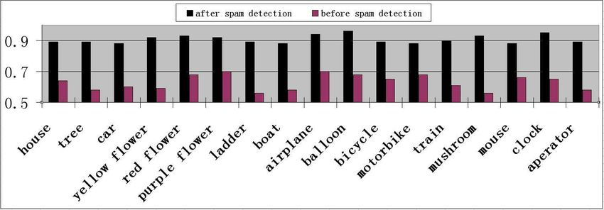
For two given image topics Ci and Cj , their visual simi-
larity context γ(Ci , Cj ) is defined as:
1 X X
γ(Ci , Cj ) = [κ̂(u, v) + κ̄(u, v)] (22)
2|Ci ||Cj |
u∈Ci v∈Cj
where |Ci | and |Cj | are the numbers of the weakly-tagged
images for the image topics Ci and Cj , κ̂(u, v) is the kernel-
based visual similarity context between two weakly-tagged
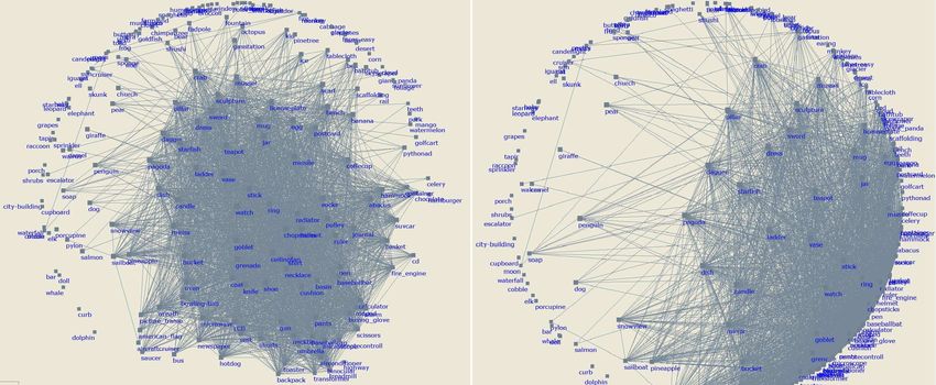
Figure 3: Different views of our topic network.
images u and v by using the kernel weights for the image
topic Ci , and κ̄(u, v) is the kernel-based visual similarity
By performing random walk over the cluster correlation
context between two weakly-tagged images u and v by us-
network, our relevance score refinement algorithm can re-
ing the kernel weights for the image topic Cj .
rank the relevance between the image clusters and the im-
The co-occurrence correlation β(Ci , Cj ) between two
age topic C more precisely. Thus the top-k image clusters,
image topics Ci and Cj is defined as:
which have higher relevance scores with the image topic,
are selected as the most relevant image clusters for the given P (Ci , Cj )
image topic C. Through integrating the cluster correla- β(Ci , Cj ) = −P (Ci , Cj )log (23)
P (Ci ) + P (Cj )
tion network and random walk for relevance re-ranking, our
spam tag detection algorithm can filter out the junk images where P (Ci , Cj ) is the co-occurrence probability for two
effectively as shown in Fig. 1(b) and Fig. 2(b). By filtering image topics Ci and Cj , P (Ci ) and P (Cj ) are the occur-
out the junk images, we can automatically create large-scale rence probability for the image topics Ci and Cj .
training images with more reliable labels to learn more ac- The cross-modal inter-topic correlation between two im-
curate classifiers for object detection and scene recognition. age topics Ci and Cj is finally defined as:
ϕ(Ci , Cj ) = α · γ(Ci , Cj ) + (1 − α) · β(Ci , Cj ) (24)
5. Cross-Modal Tag Cleansing
where α is the weighting factor and it is determined through
The appearance of synonyms may result in insufficient im- cross-validation. The topic network for our image collec-
age collections, which may prevent the underlying machine tions is shown in Fig. 3, where each image topic is linked
learning techniques from learning reliable classifiers for the with multiple most relevant image topics with larger values
synonymous image topics. On the other hand, the appear- of ϕ(·, ·).
ance of polysems may result in the image sets with huge Our K-way min-max cut algorithm is further performed
visual diversity, which may also prevent the underlying ma- on the topic network for topic clustering, thus the synony-
chine learning tools from learning precise classifiers for the mous topics are grouped into the same cluster and can be
polysemous image topics. To leverage large-scale weakly- combined as one super-topic. The images for these synony-
tagged images for computer vision tasks, it is very attrac- mous topics may share similar visual properties and seman-
tive to develop cross-modal tag cleansing techniques for ad- tics, thus they are combined and assigned to the super-topic
dressing the issues of synonyms and polysems more effec- automatically and a more comprehensive set of the relevant
tively. images can be obtained. Multiple tags for interpreting these
synonymous topics are combined as one unified phrase for
5.1 Combining Synonymous Topics tagging the super-topic. Through combining the synony-
mous topics and their similar images, we can obtain more
When people tag their images, they may use multiple text sufficient images to achieve more reliable learning of the
terms with similar meanings to tag their images alterna- classifier for the corresponding super-topic.
tively. Thus the image tags are inter-related and such inter-
related tags and their relevant images should be consid-
5.2 Splitting Polysemous Topics
ered jointly. Based on this observation, a topic network is
constructed automatically for characterizing such inter-tag Some image topics may be polysemous, which may result
(inter-topic) similarity contexts more precisely. Our topic in large amounts of ambiguous images with diverse visual
network consists of two key components: (a) a large number properties. Using the ambiguous images for classifier train-
of image topics; and (b) their cross-modal inter-topic corre- ing may result in the classifiers with high variance and low
lations. The cross-modal inter-topic correlations consist of generalization ability. To address the issue of polysemes,
two components: (1) inter-topic co-occurrence correlations; automatic image clustering is performed to split the poly-
and (2) inter-topic visual similarity contexts. semous topics by partitioning their ambiguous images into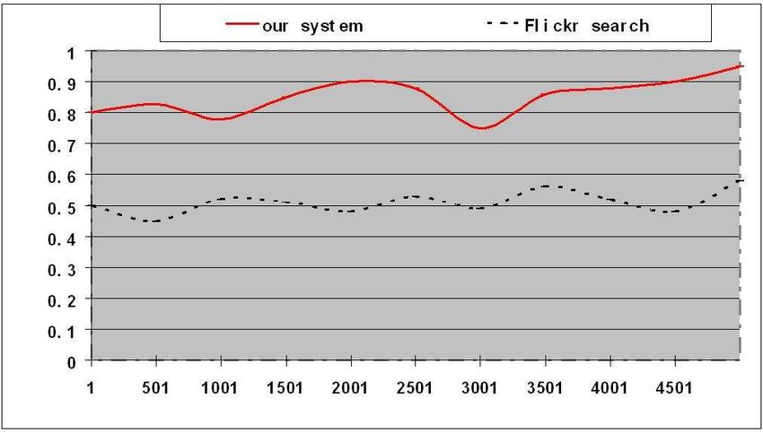
multiple clusters with more homogeneous visual properties.
Thus our K-way min-max cut algorithm is used to partition
the ambiguous images under the same polysemous topic
into multiple groups automatically and each group may cor-
respond to one certain sub-topic with more homogeneous
visual properties and smaller semantic gap.
    To address the issue of the polysemous topics more ef-        Figure 4: The comparison on the precision rates after and
fectively, WordNet is first incorporated to identify the can-     before performing spam tag detection.
didates of the polysemous topics. For a given candidate of
the polysemous topics P , all its weakly-tagged images are
first partitioned into multiple clusters according to their vi-
sual similarity contexts by using our K-way min-max cut
algorithm. The visual diversity Ω(P ) for the given candi-
date P is defined as:
                                                   2
                       X         µ(Gi ) − µ(Gj )
           Ω(P ) =                                        (25)
                                 σ(Gi ) + σ(Gj )
                     Gi ,Gj ∈P
                                                                  Figure 5: The comparison on the recall rates after and before
where µ(Gi ) and µ(Gj ) are the means of the image clusters       merging the synonymous topics.
Gi and Gj , σ(Gi ) and σ(Gj ) are the variances of the image
clusters Gi and Gj .                                              where ϑ is the set of images that are relevant to the given
    The candidates with large visual diversity between their      image topic and are returned correctly, ξ is the set of images
images are treated as the polysemous topics and are fur-          that are irrelevant to the given image topic and are returned
ther partitioned into multiple sub-topics. For a given poly-      incorrectly, and ν is the set of images that are relevant to the
semous topic, all its ambiguous images are partitioned into       given image but are not returned. In our experiments, only
multiple clusters automatically, and each cluster may corre-      top 200 images are used for calculating the precision and
spond to one certain sub-topic. By assigning the ambiguous        recall rates.
images for the polysemous topic into multiple sub-topics,             The precision rate is used to characterize the accuracy of
we can obtain multiple image sets with more homogeneous           our system for finding the particular images of interest, thus
visual properties, which may have better correspondences          it can be used to assess the effectiveness of our spam tag
between the tags (i.e., sub-topics) and the image semantics       detection algorithm. As shown in Fig. 4, one can observe
(i.e., smaller semantic gaps). Through splitting the poly-        that our spam tag detection algorithm can filter out the junk
semous topics and their ambiguous images, we can obtain:          images effectively and result in higher precision rates for
(a) multiple sub-topics with smaller semantic gaps and vi-        image retrieval. On the other hand, the recall rate is used to
sual diversity; and (b) more precise image collections (with      characterize the efficiency of our system for finding the par-
smaller visual diversity) which can be used to achieve more       ticular images of interest, thus it can be used to assess the
accurate learning of the classifiers for multiple sub-topics      effectiveness of our cross-modal tag cleansing algorithm on
with smaller semantic gaps.                                       addressing the issue of synonymous tags. As shown in Fig.
                                                                  5, one can observe that our cross-modal tag cleansing algo-
6. Algorithm Evaluation                                           rithm can combine the synonymous topics and their similar
                                                                  images effectively and result in higher recall rates for image
We have carried out our experimental studies by using             retrieval.
large-scale weakly-tagged Flickr images. We have down-                To evaluate the effectiveness of our cross-modal tag
loaded more than 10 million Flickr images. Our algorithm          cleansing algorithm on dealing with the polysemous tags,
evaluation work focuses on evaluating how well our tech-          we have compared the performance differences on the pre-
niques can address the issues of spams, polysemes and syn-        cision rates before and after separating the polysmous tags
onyms. To evaluate the performance of our algorithms on           and their ambiguous images. Some results are shown in Fig.
spam tag detection and cross-modal tag cleansing, we have         6, one can obtain that our cross-modal tag cleansing algo-
designed an interactive system for searching and exploring        rithm can tackle the issue of polysemous tags effectively.
large-scale collections of Flickr images. The benchmark           By splitting the polysemous topics and their ambiguous im-
metric for algorithm evaluation includes precision ρ and re-      ages into multiple sub-topics, our system can achieve higher
call % for image retrieval. They are defined as:                  precision rates for image retrieval.
                  ϑ                          ϑ                        We have also compared the precision and recall rates
            ρ=       ,                 %=                 (26)    between our system (i.e., which have provided techniques
                 ϑ+ξ                        ϑ+ν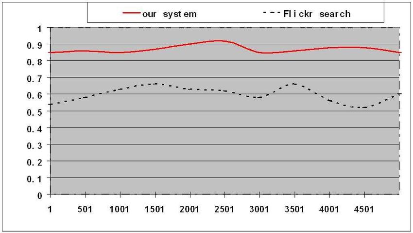
images have provided very positive results. We will also
                                                                lease our image sets with more reliable labels on our web
                                                                site.

                                                                References
Figure 6: The precision rates for some query terms before and   [1] A.W.M. Smeulders, M. Worring, S. Santini, A. Gupta and R.
after separating the polysemous topics and their ambiguous          Jain, “Content-based image retrieval at the end of the early
images.                                                             years”, IEEE Trans. on PAMI, 2000.

                                                                [2] J. Fan, C. Yang, Y. Shen, N. Babaguchi, H. Luo, “Leveraging
                                                                    large-scale weakly-tagged images to train inter-related classi-
                                                                    fiers for multi-label annotation”, Proc. of first ACM workshop
                                                                    on Large-scale multimedia retrieval and mining, 2009.

                                                                [3] Flickr, http://www.flickr.com.

                                                                [4] R. Fergus, P. Perona, A. Zisserman, “A visual category filter
                                                                    for Google Images”, ECCV, 2004.
Figure 7: The precision rates for 5000 query terms: (a) our     [5] T. Berg, D. Forthy, “Animals on the Web”, IEEE CVPR, 2006.
system; (b) Flickr search.
                                                                [6] L. Li, G. Wang, L. Fei-Fei, “OPTIMOL: automatic online pic-
to deal with the critical issues of spam tags, synonymous           ture collection via incremental model learning”, IEEE CVPR
tags, and polysemous tags) and Flickr search system (which          2007.
have not provided techniques to deal with the critical issues   [7] F. Schroff, A. Criminisi, A. Zisserman, “Harvesting image
of spam tags, synonymous tags and polysemous tags). As              databases from the web”, IEEE ICCV, 2007.
shown in Fig. 7 and Fig. 8, one can observe that our system
can achieve higher precision and recall rates for all these     [8] B.C. Russell, A. Torralba, R. Fergus, W.T. Freeman, “80 mil-
5000 queries (i.e., 5000 tags of interest in our experiments)       lion tiny images: a large dataset for non-parametric object
by addressing the critical issues of spams, synonyms and            and scene recognition”, IEEE Trans. on PAMI, vol.30, no.11,
polysemes effectively.                                              2008.

                                                                [9] K. Barnard, M. Johnson, ”Word sense disambiguation with
7. Conclusions                                                      pictures”, Artificial Intelligence, vol. 167, pp. 13-30, 2005.

                                                                [10] J. Yuan, Y. Wu, M. Yang, “Discovery of collocation patterns:
The objective of this work is to create large amounts of            from visual words to visual phrases”, IEEE CVPR, 2007.
training images with more reliable labels for computer vi-
sion tasks by harvesting from large-scale weakly-tagged im-     [11] C. Ding, X. He, H. Zha, M. Gu, H. Simon, “A Min-max
ages. A novel cross-modal tag cleansing and junk image              Cut Algorithm for Graph Partitioning and Data Clustering”,
filtering algorithm is developed by integrating both the vi-        ICDM, 2001.
sual similarity contexts between the images and the seman-      [12] J Shi, J Malik, “Normalized cuts and image segmentation”,
tic similarity contexts between their tags for cleansing the        IEEE Trans. on PAMI, 2000.
weakly-tagged images and their social tags. Our exper-
iments on large-scale collections of weakly-tagged Flickr       [13] J. Zhang, M. Marszalek, S. Lazebnik, C. Schmid, “Local fea-
                                                                    tures and kernels for classification of texture and object cate-
                                                                    tories: A comprehensive study”, Intl. Journal of Computer
                                                                    Vision, vol.73, no.2, 2007.

                                                                [14] J. Fan, Y. Gao, H. Luo, ““Integrating concept ontology and
                                                                    multi-task learning to achieve more effective classifier train-
                                                                    ing for multi-level image annotation”, IEEE Trans. on Image
                                                                    Processing, vol. 17, no.3, pp.407-426, 2008.

                                                                [15] W. Hsu, L. Kennedy, S.F. Chang, “Video search reranking
                                                                    through random walk over document-level context graph”,
                                                                    ACM Multimedia, 2007.
Figure 8: The recall rates for 5000 query terms: (a) our sys-
tem; (b) Flickr search.
You can also read