Housing Demand and Remote Work - John Mondragon - Johannes Wieland
←
→
Page content transcription
If your browser does not render page correctly, please read the page content below
Housing Demand and Remote Work
                                                                                         ∗

                     John Mondragon†                                 Johannes Wieland‡
        Federal Reserve Bank of San Francisco                          UCSD and NBER

                                          September 2022

                                                Abstract

          We show that the shift to remote work explains over one half of the record 23.8
       percent national house price increase from 2019 to 2021. Using variation in remote work
       exposure across U.S. metropolitan areas we estimate that an additional percentage
       point of remote work causes a 0.98 percent increase in house prices after controlling
       for negative spillovers from migration. This finding reflects an aggregate increase in
       demand for home space: remote work causes a similar increase in residential rents, a
       decline in commercial rents, a greater increase in prices for larger homes, and a decline
       in household size among movers. The cross-sectional effect on house prices combined
       with the aggregate shift to remote work implies that remote work raised aggregate U.S.
       house prices by 16.0 percent. Using a model of remote work and location choice we
       argue that this estimate is a lower bound on the aggregate effect. Our results argue
       for a fundamentals-based explanation for the recent increases in housing costs over
       speculation or financial factors, and that the evolution of remote work is likely to have
       large effects on the future path of house prices and inflation.

       Keywords: work from home, remote work, housing, migration, aggregation
       JEL: G5, R31, R22, E31

   ∗
      The views expressed here are those of the authors and do not necessarily reflect those of the Federal
Reserve Bank of San Francisco or the Federal Reserve System. We are grateful to Gus Kmetz for excellent
research assistance. We thank Elliot Anenberg (discussant), Arpit Gupta (discussant) and seminar partic-
ipants at the ECB, the FDIC, the SF Fed, Princeton, the FRS Mortgage Forum, the FRS Applied Micro
Conference, RedRock Finance, University of Copenhagen, and UCSD for helpful comments.
    †
      john.mondragon@sf.frb.org
    ‡
      jfwieland@ucsd.edu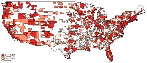
1 Introduction

U.S. house prices have grown by 23.8 percent from December 2019 to November 2021, the
fastest rate on record. At the same time, the COVID-19 pandemic has reshaped the way
households work, with 42.8 percent of employees still working from home part or full time by
November 2021 and evidence that a significant fraction of current remote work may become
permanent (Barrero, Bloom, Davis, and Meyer, 2021; Bick, Blandin, and Mertens, 2021).1 In
this paper, we show that the shift to remote work accounts for at least one half of aggregate
house price growth over this period. Our results suggests that house price growth over the
pandemic reflected a change in fundamentals rather than a speculative bubble, and that
fiscal and monetary stimulus were less important factors. This implies that policy makers
need to pay close attention to the evolution of remote work as an important determinant of
future house price growth and inflation.2
      We make three specific contributions. First, we identify a large effect of the shift to
remote work on house price growth in the cross section of U.S. micro- and metropolitan areas
(CBSAs) using exposure to the propensity for remote work. We measure exposure using the
pre-pandemic remote work share, which we argue based on pre-trends and extensive controls
is plausibly exogenous to other housing demand and supply shocks over the pandemic. We
show similarly-sized effects of remote work on residential rent growth, much smaller effects
on local inflation, and negative effects on commercial rents, consistent with remote work
increasing the relative demand for housing.
      Second, we isolate the share of the cross-sectional effect that represents an increase in
housing demand and use it to extrapolate to the aggregate effect of remote work on house
prices. Our initial estimate reflects both the increase in housing demand from working
remotely and the reallocation of housing demand through migration towards areas suited
  1
    Also see https://news.gallup.com/poll/355907/remote-work-persisting-trending-permanent.aspx.
  2
    See Bolhuis, Cramer, and Summers (2022) on how pandemic house price and rental price growth are
expected to increase inflation in 2022 and 2023.

                                                1
for remote work. We show that we can isolate the aggregate increase in housing demand
by adding high-quality controls for migration to our cross-sectional regression. We find that
the increase in housing demand accounts for two thirds of the total effect of remote work
on house prices. It also substantially increases the price of large homes relative to small
homes and reduces household size among movers. The cross-sectional estimate conditional
on migration implies that the aggregate shift to remote work accounts for at least one half
of the total increase in aggregate house prices.
Third, we build a model of location choice, remote work, and housing demand as a
laboratory to validate our aggregation approach. We calibrate the model to match the
cross-sectional distribution of remote work before and during the pandemic, and show that
it closely matches the distribution of house price growth over the pandemic. The model
implies that our extrapolation from cross-sectional estimates after controlling for migration
yields a lower bound on the aggregate effect of remote work on house prices. This shows
that our approach of controlling for negative spillovers from migration is a novel solution to
aggregating from cross-sectional estimates (Nakamura and Steinsson, 2018; Chodorow-Reich,
2019, 2020). The model also suggests that the vast majority of the increase in house prices
will persist with remote work even as housing supply normalizes.
Our results rest on credibly identifying variation in remote work that is plausibly exoge-
nous to housing demand and supply shocks from 2019 to 2021. We show that variation in
pre-pandemic remote work reflects the local distribution of occupations and their propen-
sity for remote work as well as characteristics that make remote work attractive, such as
cheap housing and amenities. In this sense the pre-pandemic remote share summarizes a
CBSA’s exposure to the increasing availability of remote work. Consistent with this inter-
pretation, we document that the pre-pandemic share of remote work is robustly correlated
with the increase in remote work over the pandemic, even conditional on important local
characteristics.
We then show that areas with more exposure to remote work saw significantly higher
2house price growth over the pandemic. Each additional percentage point of pre-pandemic
remote work implies an additional 1.97 percentage points of house price growth. Exposure
to remote work is uncorrelated with shocks to the labor market and important local char-
acteristics, and there is no evidence of pre-pandemic trends in house prices correlated with
exposure to remote work. All of this suggests that pre-pandemic exposure to remote work
provides useful exogenous variation in remote work over the pandemic.
We use the pre-pandemic remote share as an instrument for the remote work share
from the 2020 American Community Survey (ACS). More recent data on remote work with
sufficient coverage at the CBSA level is not available, but we show that the 2020 ACS remote
share correlates strongly with the broader remote work measures from Barrero, Bloom, Davis,
and Meyer (2021) and Bick, Blandin, and Mertens (2021) at higher levels of aggregation in
2020 and 2021. We estimate that an additional percentage point of remote work in 2020
increases house price growth from December 2019 to November 2021 by 1.37 percentage
points according to our preferred specification. Adding a broad range of controls, including
density, demographic characteristics, labor market indicators, and stock market exposure
leaves this estimate essentially unchanged. Additional evidence that this effect represents an
increase in housing demand caused by remote work comes from the nearly identical effects
on residential rents, negative and zero effect on commercial rents and inflation, and positive
effects on the growth of residential building permits. These results rule out two kinds of
alternative explanations. One in which a uniform demand shock, such as low interest rates,
interacts with differential housing supply elasticities across CBSAs. And a second in which
heterogenous demand shocks across CBSAs, such as labor market or financial wealth shocks,
affect housing and non-housing prices similarly.
The total effect of remote work on house prices in the cross-section captures both the
overall increase in housing demand and the reallocation of housing demand across regions
resulting from migration. We cannot directly aggregate from this cross-sectional estimate
3because migration is a quantitatively important negative “spillover” in our setting:3 House
prices will grow faster in cities attractive to remote work as migrants move in, while house
prices will grow slower in the cities losing migrants. Thus, our cross-sectional estimate of
remote work will be inflated by this negative spillover across CBSAs, and give a misleadingly
large estimate of the aggregate effects of remote work.
We show we can isolate the effect of remote work on housing demand by explicitly con-
trolling for the effects of migration on house prices in our cross-sectional regression. This
requires a precise measure of migration across CBSAs. We use address changes in the
FRBNY / Equifax Consumer Credit Panel, a 5 percent sample from the universe of con-
sumer credit reports, which allows us to observe anonymized addresses down to the census
block at a monthly frequency.
We find that the shift in demand accounts for around two thirds of the total cross-
sectional effect of remote work on house price growth. Thus, an additional percentage point
of remote work in 2020 increases house price growth from December 2019 to November 2021
by 0.98 percentage point, holding net migration fixed. Supporting our interpretation that
this effect is capturing a large increase in the demand for home space, we also show that
remote work causes a 40 percent greater house price appreciation for large houses relative
to small houses and a substantial decline in household size among movers.
To determine the effects of remote work on aggregate house prices, we combine our cross-
sectional effect on house prices that controls for migration with the aggregate shift to remote
work. This calculation implies that remote work increased house prices by 16.0 percentage
points relative to the average increase of about 23.8 percentage points, or more than one
half of the total increase. Remote work was therefore not only an important determinant of
house price growth in the cross-section, but also for the aggregate U.S. economy.
We validate our novel approach to aggregation in a spatial general equilibrium model
3
A spillover occurs when the treatment of one unit affects the potential outcome of another unit
(Chodorow-Reich, 2020).
4of location choice, remote work choice, and housing demand.4 We calibrate the model to
match the cross-sectional distribution of remote work, occupations, migration, and our cross-
sectional estimates. The model performs well in predicting house price growth in the cross-
section of CBSAs, and its predicted effect of migration on house prices is very close to that in
the data. Across a wide range of plausible parameterizations of the model, we show that our
extrapolation from the cross-sectional estimate that controls for migration is a lower bound
on the true aggregate effect of remote work on house prices. By contrast, extrapolating
from cross-sectional estimates that do not control for migration would overstate the true
aggregate effects of remote work. We then use the model to ask how much of the increase
in house prices persists assuming that remote work persists but housing supply normalizes.
Our baseline calibration implies that the vast majority of the increase in house prices—13.0
percentage points—will be permanent.
We conclude that the shift to remote work induced by the pandemic caused a large
increase in housing demand. This suggests a fundamentals-based explanation for the most
rapid increase in house prices on record, and that the future of remote work may be critical
for the path of housing demand and house prices going forward.
1.1 Related Literature
There is a rapidly growing literature on the feasibility and impact of remote work, particularly
over the pandemic period. Bartik, Cullen, Glaeser, Luca, and Stanton (2020) and Dingel and
Neiman (2020) study the actual and potential scope of remote work in the pandemic. Haslag
and Weagley (2021) analyze the patterns of migration induced by remote work and Althoff,
Eckert, Ganapati, and Walsh (2021) link the out-migration from large areas facilitated by
remote work to job losses in local non-tradables. Davis, Ghent, and Gregory (2021) study
the long-run implications of the shift to remote work.
Our work is closely related to several other studies of housing over the pandemic. Gamber,
4
See Moretti (2011) for a textbook treatment. Seminal contributions include Rosen (1979) and Roback
(1982).
5Graham, and Yadav (2021) use variation in pandemic severity combined with occupational
exposure to work from home to show that house prices increase when more time is spent
at home. Using a general equilibrium heterogeneous agent model, they argue that this
mechanism can explain a 3 percent increase in house prices from 2019-2021, about half
of the total within-model increase in prices. We instead estimate the causal effect of the
persistent shift to remote work on house price growth, show that this estimate aggregates to
a lower bound when controlling for migration, and conclude that remote work explains at
least one half of aggregate house price growth from 2019-2021. Brueckner, Kahn, and Lin
(2021) focus on the reallocation of households across locations facilitated by the move to
remote work, finding evidence that workers moved to cheaper locations from more expensive
locations. Our work shuts down this effect of remote work in order to isolate the shift in
demand for housing itself. Behrens, Kichko, and Thisse (2021) use a general equilibrium
model of production with home work, allowing for remote work to affect housing demand,
and argue that remote work has a non-linear effect on productivity and strictly increases
inequality. Stanton and Tiwari (2021) study remote workers pre-pandemic and find that
remote work is associated with higher housing expenditure shares, driven by demand for
both larger and higher quality housing, consistent with the evidence we provide.
A number of related papers have documented the effects of the pandemic and remote
work on housing and real estate markets within metro areas. Gupta, Mittal, Peeters, and
Van Nieuwerburgh (2021) and Ramani and Bloom (2021) show that housing demand shifted
from city centers to the periphery, similar to Liu and Su (2021) who show shifts in demand
consistent with a reduced demand for density. These results are consistent with Delventhal,
Kwon, and Parkhomenko (2021) who study the effects of work from home in a quantitative
framework and find migration out of the city center. Gupta, Mittal, and Van Nieuwerburgh
(2022) show that firms with a larger fraction of remote job postings reduced their demand
for office space by more.
The rapid acceleration of house price growth in the pandemic has been interpreted by
6some observers as a sign of a new U.S. housing bubble (Coulter, Grossman, Martı́nez-Garcı́a,
Phillips, and Shi, 2022). We instead argue that the large increases in house prices over the
pandemic reflect a fundamental increase in housing demand due to remote work. A related
literature examines the role of fundamentals and bubbles in the evolution of house prices
before the pandemic (see e.g., DeFusco, Nathanson, and Zwick, 2017; Kaplan, Mitman, and
Violante, 2020; Chodorow-Reich, Guren, and McQuade, 2021, for recent contributions).
Finally, we contribute to the literature aggregating from micro estimates to macro ef-
fects(see e.g., Nakamura and Steinsson, 2014; Mondragon, 2018; Chodorow-Reich, 2019;
Beraja, Fuster, Hurst, and Vavra, 2019; Herreño, 2020; Orchard, Ramey, and Wieland,
2022). Chodorow-Reich (2020) recommends using economic theory to sign the general equi-
librium effects and bound the aggregate effect, thereby avoiding heavy dependency on model
assumptions. In our analysis important general equilibrium forces pull in opposite direc-
tions: whereas migration has a negative spillover to regions with lower remote work share,
the housing wealth effect imparts a positive spillover through trade linkages (Guren, McKay,
Nakamura, and Steinsson, 2021; Stumpner, 2019). We propose to directly control for the
negative general equilibrium spillover (migration in our case), making the resulting cross-
sectional estimate a lower bound on the aggregate effect without the need of additional model
structure. We verify this approach in a spatial equilibrium model with migration.5
2 Data
We use core-based statistical areas (CBSAs) as our unit of observation. A CBSA collects
counties into economically-connected units, including both the urban core(s) and associated
periphery. This unit of observation already aggregates the effect of remote work on shifting
housing demand between the core and the periphery (Ramani and Bloom, 2021; Gupta, Mit-
tal, Peeters, and Van Nieuwerburgh, 2021), which is convenient for our purpose of estimating
5
Adao, Arkolakis, and Esposito (2019) show how to discipline all general equilibrium effects by estimating
a full set of spatial linkages. This approach requires specifying a structural model, but it allows one to recover
an aggregate point estimate rather than a lower bound.
7the effect of remote work on aggregate housing demand. Our final dataset has 895 CBSAs.
Zillow house price indices are our baseline measure of house prices.6 We measure pre-
pandemic price growth from December 2018 to December 2019, and pandemic price growth
from December 2019 to November 2021. Table 1 shows that average house price growth
increased from 4.1 percent pre-pandemic to 20.0 percent in the pandemic. Using population
weights, house price growth increased from 3.0 percent to 23.8 percent. While the pandemic
house price growth is measured over a longer period of time, the annualized growth rate of
11.3 percent is still well above the pre-pandemic growth rate.
We obtain rents for a subset of 178 CBSAs from Apartment List. Similar to house prices,
rent growth accelerates dramatically from 2.4 percent in 2019 to 14.9 percent (7.2 percent
annualized) from December 2019 through November 2021.
We rely on American Community Survey data from the 2015-2019 survey waves as well
as the 2020 experimental run to measure remote work, where remote work is defined as an
employed person that does not commute.7 We also use the ACS to measure local demographic
characteristics. These data are available at the individual level with public-use microdata
area (PUMA) geographic identifiers, which we aggregate to CBSAs using the person-level
weights and PUMA-CBSA area correspondence files.8
Table 1 shows that the national (population-weighted) remote worker share increased
from an average of 5.2 percent before the pandemic to 16.3 percent in 2020. Other surveys
report higher remote shares: Bick, Blandin, and Mertens (2021) report more than 20 percent
of workers are remote by late 2020 while Barrero, Bloom, and Davis (2021) report that 49
percent of paid working days were done remotely at the same time. These surveys are
also able to capture the evolution of broader remote work trends such as hybrid work in
subsequent years and so would be ideal to measure remote work adoption. But they are also
relatively sparse below the state level, making them difficult to use for our analysis.
6
See https://www.zillow.com/research/data/. Our results are also robust to using the proprietary S&P
Corelogic Case-Shiller index.
7
We exclude individuals in the armed forces when calculating remote work shares.
8
See https://mcdc.missouri.edu/geography/PUMAs.html.
8To determine the relationship between the 2020 ACS remote work share and these alter-
native surveys, we construct state-level measures of the fraction of days worked remotely for
2020, 2021, and 2022 if available from Barrero, Bloom, and Davis (2021) and Bick, Blandin,
and Mertens (2021). Figure 1 shows binned scatter plots of these measures against our
measure of remote work from the ACS. There are two important takeaways. First, our ACS
measure is strongly correlated with both survey measures of remote work in all years and this
correlation is stable across years. Since these measures also explicitly capture hybrid work
arrangements, our ACS measure will also pick up the effects of hybrid work. Second, the
ACS measure tends to understate the prevalence of remote work by about 15-30 percentage
points. This implies that our empirical estimates using the ACS estimates will end up being
scaled up to reflect this discrepancy. Overall, these results show that the 2020 ACS gives a
very accurate measure of remote work in the cross-section.
Our analysis requires a high-quality measure of migration in and out of CBSAs. Here we
rely on the FRBNY/Equifax Consumer Credit Panel (Lee and Van der Klaauw, 2010). These
data, built from an anonymized 5 percent sample of the universe of consumer credit reports,
provide information on an individual’s reported address on their credit files down to the
census block level at a monthly frequency. We track an individual’s reported CBSA across
the same periods used to measure house price changes. We then aggregate these moves
into gross in- and outflows, and define net migration for CBSA i between t and t + 1 as
Gross Inflowi,t,t+1 −Gross Outflowi,t,t+1
Net Migrationi,t,t+1 ≡ Ni,t
, where N is the number of individuals
in that CBSA in the pre-period. On an annualized basis, the dispersion of migration reported
in Table 1 is quite similar in the pre- and post-pandemic periods.
We use population density (population per square mile) from the U.S. Census as a mea-
sure of the CBSA housing supply elasticity. Baum-Snow and Han (2019) extract housing
supply elasticities for new and existing housing in large metropolitan areas using labor de-
mand shocks at the census tract level. For the subsample in which both measures are avail-
able, the correlation between log density and the first principal component of their supply
9elasticities is −0.62.
We collect unemployment rates from the Local Area Unemployment Statistics (LAUS)
to measure shocks to the local labor market. We calculate the pre-pandemic unemployment
rate as the average in 2019, the pandemic unemployment rate as the average in 2020, and the
change in unemployment from November 2019 to November 2021. These choices avoid sea-
sonality issues and use the most recent date available. The average change in unemployment
over the full pandemic period is actually quite low, despite the extremely rapid increase in
early 2020, due to the very rapid recovery in labor markets. As an alternative labor market
indicator, we calculate wage growth from average wages per employee in the QCEW. The
total wage bill is reported at quarterly frequency, so we measure pandemic wage growth from
2019Q4 to 2021Q4 and pre-pandemic wage growth from 2018Q4 to 2019Q4.
To capture exposure to the growth in stock market valuations over the pandemic, we
construct the share of total dividend income in adjusted gross income by CBSA in 2019
(Chodorow-Reich, Nenov, and Simsek, 2021). This is the most recent geographically disag-
gregated data released by the IRS.
3 Empirical Results
3.1 Research Design
We use cross-sectional data to recover the effect of increased remote work on housing demand
as measured by house prices. Our baseline regression is an instrumental variables regression
of the form:
First Stage: Remote Work 2020i = κ + Xi′ θ + γRemote Work 2015-19i + ζi (1)
Second Stage: House Price Growthi = α + Xi′ δ + β Remote\
Work 2020i + ϵi (2)
10where Remote Work 2015-19i is the share of employed individuals working from home in
the 2015-2019 ACS, Remote Work 2020i is the share of employed individuals working from
home in the 2020 ACS, House Price Growthi is house price growth over the pandemic, and
X is a vector of controls.
We use an IV approach as a benchmark since unobserved shocks to housing demand
and house prices during the pandemic likely affected remote work in 2020. In fact, if remote
workers require more housing, then any shock that pushes up house prices will reduce remote
work as remote workers migrate to cheaper housing or return to office work. Our instrument
must be plausibly uncorrelated with other shocks to house prices while still being correlated
with actual remote work over the pandemic.
We use pre-pandemic remote work share, calculated over 2015-2019, as our instrument.
Intuitively, we can think of the concentration of remote work over the pandemic as reflecting
local amenities, the cost of housing, and the distribution of occupations amenable to remote
work. Table 2, where we regress pre-pandemic remote work on local observables, confirms
this insight.9 The predicted local remote share based on local occupation shares interacted
with the probability of being remote in an occupation at the national level is a very strong
predictor of pre-pandemic remote work.10 Similarly, amenities such as a mild winter climate
and low summer temperature and humidity strongly predict remote work.11 In contrast,
density is only weakly correlated with remote work, suggesting a smaller role for housing
cost in explaining the cross-sectional variation in remote work exposure.
Based on these results, we interpret the pre-pandemic remote work share as a sufficient
statistic for how exposed a location is to the availability of remote work. Once remote
work becomes available more broadly during the pandemic, these same locations will see
relatively more remote work due to both more immigration and more local workers electing
9
Table A1 shows bivariate comparisons.
10
To construct predicted remote work share we measure remote work shares for 4-digit occupation codes
in the 2015-19 ACS and then weight these occupational shares by the share of workers in that occupation
in each CBSA.
11
We draw our climate measures from https://www.ers.usda.gov/data-products/natural-amenities-scale/.
11to work remotely. This implies pre-pandemic remote work shares will be predictive of remote
work shares over the pandemic, satisfying the relevance assumption. We also check that the
exclusion restriction, that exposure to remote work is uncorrelated with other shocks to house
prices, likely holds by examining pre-trends and the stability of our estimates conditional on
important local shocks and characteristics.
If the exclusion restriction holds, then equations (1)-(2) estimate a valid causal effect
of remote work on house prices in the cross-section. However, because this causal effect
contains the effects of net migration induced by remote work across CBSAs, it may not be
appropriate for quantifying how remote work affects aggregate house prices. To the extent
that the pre-pandemic remote share captures how suitable a location is for remote work,
we would expect such locations to see net inflows of remote workers. Such migration would
raise housing demand and house prices in high remote share locations, while at the same
time lowering house prices in low remote share areas, all else equal. Therefore, migration
would raise the cross-sectional causal effect of remote work, even though aggregate housing
demand is unaffected.
In order to isolate the component of remote work that reflects a shift in aggregate housing
demand, we control for the effects of migration on remote work and house prices,
Remote Work 2020i = κ + Xi′ θ + γ1 Remote Work 2015-19i + γ2 Net Migrationi + ζi (3)
House Price Growthi = α + Xi′ δ + β1 Remote\
Work 2020i + β2 Net Migrationi + ϵi (4)
Intuitively, controlling for net migration will collect any effects remote work has on house
prices through net migration in the estimate of β2 . This means that β1 will capture the
direct effects of remote work on house prices only through the shift in housing demand.
In Appendix 1.1 we show that β1 will recover the intended effects if unobserved shocks to
migration and house prices are uncorrelated. If unobserved shocks to migration and house
prices are positively correlated, which is the more likely case, then we will understate the
12true effect of remote work on house prices.12
If we combine estimates of β1 with the representative level of remote work in 2020, we
obtain an estimate of the effect of remote work on aggregate house prices. In section 4 we
argue using a model of remote work choice and location choice that this estimate is a lower
bound on the aggregate effects of remote work.
We conservatively cluster standard errors at the state level in all specifications. CBSAs
often cross state borders, so we allocate a CBSA to the state which contains the largest share
of population. Following the recommendations by Solon, Haider, and Wooldridge (2015), we
estimate unweighted regressions and in Section 3.6 we show that treatment effects vary little
with population size.
3.2 Remote Work and House Prices
We next argue that the remote work share in 2015-2019 satisfies the relevance and exclusion
restrictions necessary for it to be a valid instrumental variable for pandemic remote work.
Figure 2 separates CBSAs into 20 bins based on their remote work share in 2015-2019
and then plots the average remote work share in 2020 within each bin, along with the linear
regression line from the underlying data. Areas that had large shares of remote work prior
to the pandemic also had significantly larger shares of remote work during the pandemic:
areas at the top of the pre-pandemic distribution have more than 15 percent of workers at
home in 2020 while areas at the bottom of the pre-pandemic distribution only have about
5 percent of workers at home in 2020. This is consistent with our argument that the same
underlying fundamentals that made a city amenable to remote work in the pre-pandemic
period continued to attract remote work during the pandemic.
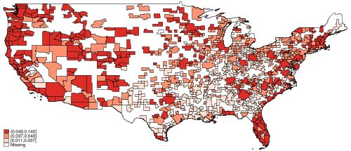
Figure A1 shows heat maps of the distribution of remote work pre-pandemic and in 2020
across CBSAs, grouping CBSAs into terciles in both periods. The stability of the tercile
membership across the two maps is suggestive of a strong first stage relationship between
12
A simple example of a shock that would induce a positive correlation would be firm creation, which
induces immigration for new jobs as well as higher incomes (and so house prices).
13pre-pandemic and pandemic remote work shares.
Column (1) of Table 3 reports the corresponding regression. For each percentage point
of remote work share in 2015-19 we expect 1.74 percentage points of remote work during
2020. The estimate is very precise with the 95 percent confidence band ranging from 1.52
to 1.95. Since the aggregate remote share increases by a factor of 3, the first stage implies
that low-remote areas get a slightly larger multiplicative treatment than high-remote areas.
Still, the r-squared of 39 percent shows that the pre-pandemic remote share captures a
substantial fraction of the variation in remote work over the pandemic, and therefore satisfies
the relevance restriction.
Columns (2) through (4) of Table 3 sequentially introduce controls for important local
observables. Column (2) adds pre-pandemic house price growth as a control. Column (3),
additionally controls for racial/ethnic and age composition, and quintiles for CBSA density.13
Column (4) controls for local labor market conditions before the pandemic and over the
course of the pandemic and for the exposure to the stock market, proxied with the share of
local income due to dividends. Introducing these controls raises the r-squared to 64 percent
and has only small effects on the pre-pandemic remote work estimate, suggesting that this
measure of remote work exposure is not correlated with other pandemic-related shocks to
areas affecting levels of remote work.
We next provide evidence that exposure to remote work satisfies the exclusion restriction
that it only affects house prices through its effect on pandemic levels of remote work. We
begin by documenting the robust and stable relationship between exposure to remote work
and house price growth over the pandemic (the reduced form). In Figure 3A we plot house
price growth over the pandemic against the remote work share in 2015-19. This shows that
pandemic house price growth is strongly positively correlated with exposure to remote work.
The areas most exposed to remote work saw house prices grow by twice as much as areas at
13
The relationship between log density and remote share is U-shaped: high-density metro areas have
similar remote shares to low-density metros, and higher remote shares than medium-density areas. There
is a similar relationship between the share of the population above 65 and remote work. To capture these
patterns we control for density and age composition nonparametrically.
14the bottom of the distribution. However, house price growth was very high across the board;
even the areas least exposed to remote work saw house prices grow by about 15 percent.
It is possible that the large apparent effect of remote work on house prices simply reflects
pre-existing trends in house prices caused by differences in underlying fundamentals unrelated
to remote work. In Figure 3B we plot pre-pandemic house price growth from December 2018
to December 2019 against the remote work share in 2015-19. The relationship between
remote work and pre-pandemic house price growth is negative, though the effects are small
and not statistically significant. In Figure 4A we plot average house prices indexed to
December 2019 for terciles of exposure to remote work. House price growth across these
groups was indistinguishable leading up to the pandemic, but then began to diverge in 2020,
with the gap widening throughout 2021 as house prices continued to grow rapidly.
As a more formal test for pre-trends, Figure 4B plots the regression coefficient of house
price growth relative to December 2019 against the 2015-19 remote work share. The estimates
are not statistically distinguishable from zero at the 95 percent level before the pandemic
begins, but the estimates rapidly increase by late 2020. This shows that the differences in
house price growth correlated with exposure to remote work are not reflective of differential
trends prior to the pandemic.
The absence of pre-trends does not rule out the possibility that other shocks during
the pandemic may have increased housing demand in locations with a high pre-pandemic
remote share relative to locations with a low pre-pandemic remote share. However, any
explanation of our estimates must also be consistent with the build-up of the treatment
effect in Figure 4B. The corresponding build-up in expectations that remote work will
be permanent documented by Barrero, Bloom, and Davis (2021) provides an explanation
consistent with our hypothesis. In contrast, explanations that emphasize the pandemic, for
example a revaluation of outdoor space, would imply stronger effects on house prices in 2020
when restrictions were more widespread and vaccines were not available.
To address other possible violations of the exclusion restriction we add controls to capture
15omitted variables and examine the stability of our estimate on the effect of remote work on
house prices. Column (1) of Table 4 reports the regression without controls. A location with
a one percentage point higher remote work share in 2015-19 should expect an increase in
house price growth of 1.97 percent during the pandemic. This estimate is also fairly precise
with the 95 percent confidence band ranging from 1.36 to 2.58. Columns (2) through (4)
of Table 4 include the set of controls from Table 3. The net effect is a very slight increase
in the our estimate to 1.98, even though many of the controls themselves are statistically
significant and raise the r-squared from 17 to 39.
The stability of the remote work estimate reflects that the pre-pandemic remote share
is only weakly correlated with many controls. For example, the correlation of remote work
is −0.19 with the pre-pandemic unemployment rate, 0.06 with the change in unemployment
from 2019 to 2020, and 0.15 with the change in unemployment from November 2019 through
November 2021. Therefore, our estimate for remote work does not appear to be correlated
with a shock to labor demand. More broadly, the U.S. economy had almost returned to full
employment by November 2021, which suggests that there is limited scope for alternative
explanations based on labor demand.
3.3 The Total Effect of Remote Work
Column (5) of Table 4 reports the IV coefficient from estimating equations (1)-(2). Each
additional percentage point of remote work in 2020 implies a 1.14 percent faster house
price growth during the pandemic. The Kleibergen-Paap weak identification F-statistic is
extremely high, suggesting that the risk of weak instrument issues is low (Andrews, Stock,
and Sun, 2019). This is consistent with the high r-squared in the first stage results in Table 3,
and also yields a fairly narrow 95 percent confidence band of 0.80 to 1.47.
Columns (6) through (8) of Table 4 add our set of control variables. With our full set
of controls in column (8), we obtain a slight increase in the overall estimate to 1.37 that
remains precisely estimated with the 95 percent confidence bands extending from 1.05 to
161.69. The IV coefficients are roughly twice as large as their OLS counterparts, which are
displayed in Table A2. This suggests that there are significant shocks to pandemic housing
demand that negatively affect remote work and/or there is substantial measurement error
in the 2020 remote work share.14
If remote work causes an increase in overall demand for housing services then we should
also expect to see an effect of remote work on rents over the pandemic. We now turn to the
subsample of 178 CBSAs for which we have rental index data. For brevity we only report
the IV estimate with all controls included — equivalent to column (8) of Table 4. In the
appendix we include a full set of regressions of the first stage (Table A3) and the reduced
form and IV regressions Table A4.
Row (1) of Table 5 reports the IV estimate for pandemic rent growth. It implies that
an additional percentage point of remote work in 2020 increases rent growth from December
2019 to November 2021 by 1.09 percentage points. This estimate is very close to our baseline
estimate for house price growth (1.37 percentage points) and almost identical to the estimate
for house price growth in this sub-sample (1.03 percentage points as shown in row (2) of
Table 5).
A further way to assess whether there was a housing-specific increase in demand is to
check whether the price of housing has increased relative to non-residential real estate or the
broader bundle of consumer expenditures. If demand for residential real estate has partly
reflected substitution away from commercial real estate, then we should expect to see lower
commercial real estate prices in areas with more remote work. Alternatively, if the growth in
house prices is driven by some common shock to real estate values (such as accommodative
monetary policy), then we should expect to see similar trends across all types of real estate.
We test this prediction using commercial rent data from REIS for 25 CBSAs and Bureau of
Labor Statistics price indices for 22 CBSAs.15 Given the small sample size we report reduced
14
Rothbaum, Eggleston, Bee, Klee, and Mendez-Smith (2020) document the potential for nonresponse bias
in the 2020 ACS production run due to the pandemic. To the extent that this measurement error is classical,
our IV estimates are asymptotically unaffected. See also https://usa.ipums.org/usa/acspumscovid19.shtml
15
We use the Reis commerical real estate effective rent index, now provided by Moody’s CRE. This is a
17form regressions with lagged dependent variables as controls and robust standard errors.
Row (3) of Table 5 shows the reduced form regressions for commercial rent growth. A
one percentage point increase in remote work exposure predicts a marginally significant
−0.26 percent decline in pandemic commercial rents. Row (4) reports the corresponding
estimates for house price growth in the same sub-sample: a one percentage point increase
in remote work exposure predicts a 2.37 percent increase in house prices, which is highly
statistically significant and consistent with the broader sample. The house price growth
effects are roughly ten times larger in magnitude and have the opposite sign as the effects on
commercial rents. Thus, the data provide evidence for substitution from office space to home
space. The relatively small decline in the office rent index may reflect that it captures both
existing and new leases, whereas our housing price and residential rent series only reflect
new purchases and leases.
A related concern is that increasing housing costs are reflective of a broader increase
in prices faced by consumers. Row (5) of Table 5 displays the reduced form regression for
the pandemic inflation rate excluding shelter on the remote worker share. The price level
excluding shelter grows by 0.44 percent more over two years for every percentage point of
initial remote work exposure, a statistically insignificant effect. For comparison, the effect
of remote work exposure on house price growth in the same sub-sample is 2.98 percentage
points (row 6). The insignificant inflation response is thus roughly one seventh the magnitude
of the very significant house price responses. This corroborates our claim that remote work
triggered a relative increase in the demand for housing and thus an increase in the relative
price of housing.
Together with our results on residential and commercial rents, this finding rules out alter-
native explanations for our results based on broad-based increase in demand correlated with
remote work (e.g., an increase in financial wealth). However, another possible explanation is
that remote work exposure proxies for a low housing supply elasticity, so that even a uniform
quarterly, hedonic index intended to give the average “effective rent” per square foot for large-building office
space in the metro area.
18increase in housing demand would increase house prices more in less elastic/higher remote
work CBSAs. The fact that our estimates in Table 4 are insensitive to controlling for density
is evidence against this hypothesis. We provide further evidence against this explanation by
estimating the response of building permit growth and cumulative home sales to remote work
exposure. If differential supply constraints explain our price results, then we should expect
to see a negative relationship between remote work and permits or home sales. Row (7) of
Table 5 instead shows that housing permits grew faster in areas more exposed to remote
work.
However, these additional permits are unlikely to have been completed by the end of our
sample period: Row (8) of Table 5 shows that there is essentially no relationship between
remote work exposure and the cumulative number of homes sold in 2020-21 relative to 2018-
19. This suggests that the housing supply elasticity was essentially zero over the period we
study.
There are a number of additional local observables that are correlated with the increase
in remote work over the pandemic: the share of individuals with college education, the log
median income, climate characteristics, and census region fixed effects. We do not include
these controls in our baseline regressions because they absorb significant valid variation in
remote work, leaving the remaining variation at risk of not being representative of the true
average treatment. For example, the share of college educated workers is an important
predictor of remote work, as occupations that disproportionately employ college educated
workers tend to be more amenable to remote work. By including this control we would
restrict attention to potentially unrepresentative variation, which would be problematic for
aggregation. Similarly, Figure A1 shows that remote work is more common in the West and
less common in the South, but this is largely explained by the geographic distribution of
occupations and amenities and it is not obvious that we want to exclude this variation.
However, we check how sensitive our estimates are to including these controls. We report
the first stage, reduced form, and IV estimates with these conservative controls in Table A11
19and Table A12. The IV estimates with all controls included is now 1.76 (95 percent confidence
band from 1.20 to 2.32) versus 1.37 in our baseline regression. The first-stage is also less
powerful indicating that the variation we use is less likely to be representative of the broader
increase in remote work during the pandemic.
A closely-related question is whether specific subsets of the variation in pre-pandemic re-
mote work ultimately accounts for the effect of remote work on house prices. In Table A10, we
re-estimate our baseline equations using three distinct subsets of pre-pandemic remote work
as our instrumental variable: (1) the remote work expected by the pre-pandemic distribution
of occupations, (2) the average January and July temperatures (the most predictive climate
variables we consider), and (3) the residual of pre-pandemic remote work after partialling
out the occupation- and climate-driven variation. To ensure we isolate the particular source
of variation, we include the remaining variation in the 2015-19 remote work share as a con-
trol. We find that each source of variation implies that remote work had economically large
effects on housing markets over the pandemic. In relative terms the effects are largest for the
residual variation and smallest for occupational variation, which is in large part explained
by differential loadings on migration. The first stage F-statistics for these regressions, while
reasonably strong, are uniformly lower than what we find using pre-pandemic remote work
alone. This suggests that pre-pandemic remote work is more likely to capture variation that
will reflect the true average treatment effect we need to plausibly aggregate our effects.
3.4 Decomposing The Effect of Remote Work
The large effects of remote work on house price and rent growth that we estimate in the
cross-section reflect both an aggregate increase in housing demand, as remote work requires
more housing, as well as a relocation of housing demand towards areas that are better suited
for remote work. We expect only the former to significantly affect aggregate housing demand
and house prices. Therefore, to determine the aggregate effects of remote work we need to
separate the total effect of remote work on housing demand into these two components.
20We first document that remote share exposure is a quantitatively important determi-
nant of net migration. The binned scatter plot Figure 5 shows that exposure to remote
work is strongly correlated with net inflows over the pandemic. Table A8 reports specifica-
tions mirroring our primary results and we find that areas exposed to remote work saw much
higher net inflows of residents. These inflows were also strongly correlated with pre-pandemic
inflows, suggesting pre-existing migration patterns may have been amplified over the pan-
demic. These results suggest that migration may be a quantitatively important fraction of
the estimated effect of remote work on housing demand in the cross-section of CBSAs.
To isolate the aggregate increase in housing demand we estimate equations (3)-(4), in
which we directly control for net migration into a CBSA. Table 6 reports the reduced form
and IV estimates. The migration controls enter positively and reduce the cross-sectional
estimate of remote work on house price growth to 1.31 (reduced form, column 1) and 0.73
(IV, column 5). This is roughly a one third drop compared to our baseline estimates in
Table 4 that do not control for migration. Mechanically, the reduced form and IV results
move in similar magnitude because the first stage is essentially unchanged (Table A9). Note
that this attenuation of the remote work effect does not reflect an omitted variable bias, but
rather is an instance of a “bad control.” By controlling for migration we deliberately shut
down one of the mechanisms by which remote work exposure can affect housing demand
across locations (see Appendix 1.1 for details).16
Our estimate increases slightly after including the full set of controls (columns 3 and
7). In columns (4) and (8) we control for migration non-parametrically by including deciles
of pandemic net migration and pre-pandemic net migration. Our IV estimate of the effect
of remote work on house prices remains almost unchanged at 0.98. This suggests that this
effect is not driven by a non-linear migration response or measurement error in the migration
variable.
16
We have also run specifications in which we controlled separately for net migration among individuals
with high credit scores or originating from zip codes with high incomes. These controls had very little
additional explanatory power over our baseline net migration control.
213.5 Supporting Evidence for the Mechanism
We have argued that the effect of remote work on house prices after controlling for migration
represents an aggregate increase in the demand for home space. Here we present supporting
evidence for this interpretation using data on price indexes for houses of different sizes and
on household formation.
If housing is perfectly divisible then an increase in demand would raise the price per square
foot uniformly. However, since housing is indivisible housing demand may be segmented
across subsets of the housing stock (Piazzesi, Schneider, and Stroebel, 2020), and the remote
work shock may not fall uniformly across these segments. In particular, an increase in the
demand for more space caused by remote work likely increases the demand for large houses
more than the demand for small houses. We test this hypothesis using Zillow price indices
that are broken out according to the number of bedrooms, available for a subset of our
CBSAs. Rows (1) through (5) of Table 7 display IV estimates of the effect of remote work
on house price indices ranging from 1 to 5 bedrooms. These regressions include our full set
of controls from column (7) of Table 6. The estimates show that the effect of remote work
on house price growth is roughly 40 percent larger for houses with at least three bedrooms
compared to houses with only one bedroom. This is consistent with the argument that
remote work increases the demand for space.
Another margin of adjustment is for remote workers to reduce the size of the household
itself. For example, people who lived with roommates prior to the pandemic may decide to
live alone with the onset of remote work, thus reducing their household size and increasing
their total demand for home space. We construct measures of the number of adults in each
primary sample member’s household, defined as individuals with the same anonymized ad-
dress, in the FRBNY/Equifax Consumer Credit Panel.17 We then calculate the log change in
17
For each primary sample member, the FRBNY/Equifax Consumer Credit Panel provides credit reports
all individuals using the same address in their credit reports, even if they are not in the primary sample. To
minimize erroneous household counts from non-traditional arrangements, like military bases or dorms, we
drop any household with more than 7 adult members.
22household size over the pre-pandemic and pandemic periods, distinguishing between house-
holds that moved or stayed in the same location.
Distinguishing between movers and stayers is important because of local general equilib-
rium effects: to the extent that the local housing supply is fixed in the short-run and we hold
population fixed by controlling for net migration, we would not expect to see any change in
average household size in a CBSA. We therefore test whether movers in high remote work
areas choose to reduce their household size by more than movers in low remote work ar-
eas. Here we interpret movers as the marginal buyers or renters in the housing market and,
in this sense, we test for a greater demand for space among the marginal buyer. In local
general equilibrium, we expect that any such effect will at least be partly offset by stayers
maintaining a correspondingly larger household size.
Rows (6)-(8) of Table 7 report the IV estimates of the effect of remote work on household
size according to move status, again conditional on our full set of controls. Row (6) shows
that remote work only modestly and insignificantly reduces household size over the pandemic,
with the IV estimate showing an elasticity of −0.03. This is consistent with a relatively fixed
housing supply and adult population in a CBSA conditional on our controls.
When we break these numbers up into households that moved (both into and within
the CBSA) and households that did not move at all, we find that movers in areas more
exposed to remote work reduce the sizes of their households. The estimate for movers in
row (7), −0.18, implies that remote work reduced the average household size of movers by
−0.18×16.3=−2.9 percent.18
Row (8) shows that there is a positive but weaker relationship between remote work and
changes in household size for households that did not move, consistent with stayers absorbing
the remote work shock by increasing their household size. We also find that net inflows from
December 2019 to November 2021 are strongly positively correlated with household size for
all households, consistent with the view that housing supply was relatively fixed (Table A13).
18
Table A14 shows that the negative effect on household size among movers reflects an increased probability
of reducing household size.
23These results support the claim that remote work increased housing demand. This in-
creased demand translated into more house price growth for larger houses as well as reduc-
tions in household size, concentrated among households that moved across or within CBSAs.
3.6 Aggregation
We now use our cross-sectional effects on house prices cleansed of the migration channel
(Table 6) to estimate the aggregate effect of the shift to remote work on house prices. For
extrapolation we use the estimates in column (8) with all controls included.
The weighted 2020 remote worker share for the U.S. economy is 16.3 percent. Mul-
tiplying this value with our IV estimate in column (8), we obtain an aggregate effect of
16.3×0.98=16.0 percent. Since aggregate house prices grew by 23.8 percent from December
2019 to November 2021, our IV estimate implies that remote work can explain 16.0/23.8=67
percent of the total increase in house prices over the pandemic. In the following section 4,
we argue that this extrapolation represents a lower bound on the aggregate effect because
we control for the effect of migration in the cross-section.
For the purpose of aggregation it is important that our treatment effects are nationally
representative. Following Solon, Haider, and Wooldridge (2015) we estimate the effects of
remote work on house prices by population decile. Figure A2 shows that the treatment effects
vary little by population. Using the population in each decile as weights, the weighted effect
of remote work on house prices is 1.00, essentially identical to our baseline estimate.19
4 Model
We now use a model of housing demand, location choice, and work mode choice to show that
extrapolating from our cross-sectional estimate that controls for migration provides a lower
bound on the aggregate effect.
19
We can also extrapolate by multiplying the ten treatment effects with the 2020 remote work share in
each decile. This yields an aggregate effect of remote work on house prices of 16.6%.
24The model deliberately omits channels that generate positive spillovers across locations,
such as trade spillovers from positive housing wealth effects (Guren, McKay, Nakamura,
and Steinsson, 2021; Stumpner, 2019). Adding such channels would only strengthen the
argument that our cross-sectional estimate that controls for migration constitutes a lower
bound on the aggregate effect. Our model also omits aggregate general equilibrium effects
through monetary policy. The model therefore provides an estimate for the effect of remote
work on house prices holding monetary policy fixed.
4.1 Firms and Workers
There is a set of locations l = 1, ..., L and occupations o = 1, ..., O. Within each location
there are firms indexed by f . Firms are immobile with ℓ(f ) denoting the location of firm
f . Firms only employ workers of a single occupation, o(f ), at an occupation-specific wage
zo(f ) . Firms are perfectly competitive and production is linear in labor, so that zo(f ) is also
the value of output produced by a worker at firm f .
Workers have fixed occupations and a fixed attachments to firms. Each worker attached
to firm f can choose to either work in the office of firm f (and thus in location ℓ(f )), work
remotely in location ℓ(f ), or work remotely in another location l ̸= ℓ(f ). The work mode
and location decision is an optimization problem based on location amenities, prices, and
idiosyncratic tastes. Workers consume a non-housing good c and a housing good h.
4.2 Consumption Decision
We first solve for the optimal goods bundle (c, h) given attachment to firm f , and given the
choices of location l and work mode w (remote r or office b).
The utility function is CES, with weight θw on the housing good and elasticity of substi-
tution ζ between housing and non-housing:
ζ
ζ−1
ζ−1 1 ζ−1
1
ζ ζ ζ
Uf lw = (1 − θw ) cf lw + θw hf lw
ζ
25You can also read