Implementation of Airy function using Graphics Processing Unit (GPU)
←
→
Page content transcription
If your browser does not render page correctly, please read the page content below
ITM Web of Conferences 32, 03052 (2020)                                                     https://doi.org/10.1051/itmconf/20203203052
ICACC-2020

      Implementation of Airy function using Graphics
                 Processing Unit (GPU)

                Yugesh C. Keluskar1 , Megha M. Navada2 , Chaitanya S. Jage3 and Navin G. Singhaniya4
                                         Department of Electronics Engineering,
                                         Ramrao Adik Institute of Technology,
                                                 Nerul, Navi Mumbai.
 Email : yugeshkeluskar.yk@gmail.com1 , meghanavada@gmail.com2 , chaitanya.jage@rait.ac.in3 , navin.singhaniya@rait.ac.in4

    Abstract—Special mathematical functions are an integral part           Airy function is the solution to Airy differential equa-
of Fractional Calculus, one of them is the Airy function. But          tion,which has the following form [22]:
it’s a gruelling task for the processor as well as system that is
constructed around the function when it comes to evaluating the
special mathematical functions on an ordinary Central Processing                                  d2 y
                                                                                                       = xy                          (1)
Unit (CPU). The Parallel processing capabilities of a Graphics                                    dx2
processing Unit (GPU) hence is used. In this paper GPU is used
to get a speedup in time required, with respect to CPU time for            It has its applications in classical physics and mainly
evaluating the Airy function on its real domain. The objective         quantum physics. The Airy function also appears as the so-
of this paper is to provide a platform for computing the special       lution to many other differential equations related to elasticity,
functions which will accelerate the time required for obtaining the    heat equation, the Orr-Sommerfield equation, etc in case of
result and thus comparing the performance of numerical solution        classical physics. While in the case of Quantum physics,the
of Airy function using CPU and GPU.                                    most well-known application of this equation is while solving
   Keywords- GPU, CPU, Airy function, Speedup.                         WKB approximation problem [3],[24]. Taking a few steps we
                                                                       can arrive at the Airy Differential equation as given below.
                                                                       The following is the One-Dimensional Time Independent
                                                                       Schrödinger’s equation
                      I.   I NTRODUCTION
    Fractional calculus (FC) is a field of mathematics that deals                   −h̄2 d2 ψ(x)
with derivatives and integrals of arbitrary non-integer order.                                   + V (x)ψ(x) = Enψ(x)                (2)
                                                                                    2m dx2
It is being used in engineering domain extensively due to its
ability to model real-world systems more accurately than its in-            Where ψ(x) is the wave-function, h̄ is the reduced Planck’s
teger order variant. It is a topic which is around 320 years old!.     constant (Dirac constant), m being mass of the particle, V (x)
The inception of this field can be attributed to a letter written to   is the potential function and E is the total energy. This equation
Guillaume de l’Hopital by Gottfried Leibniz in the year 1695 in        basically says that Kinetic Energy + Potential Energy = Total
which he mentions about fractional order derivatives, see [26],        Energy, and that is what each term in this equation signifies.
one can also find the foundational work of Fractional calculus         When we consider a triangular potential well i.e V (x) = qεx
in the early papers of Niels Henrik Abel [27]. But due to its          (q is charge of particle and ε is the electric field strength), we
mathematically intricate and cumbersome nature it remained             arrive at the following equation
mostly unexplored for many years until 1974 when the “First
Conference on Fractional Calculus and its Applications” was               For x > 0, n = 1, 2, ..
held at the University of New Haven,Connecticut [28]. In
recent years applications of this are growing nowadays in                           −h̄2 d2 ψ(x)
a rapid manner as there is a community of researchers that                                       + qεxψ(x) = Enψ(x)                  (3)
                                                                                    2m dx2
have came together to revive this field with the help of when
advanced computing technology [1],[2]. As mentioned before                 The above equation is the same as equation (1) with
using this mathematical technique, the scope of describing             some constant terms mugging up the equation of which the
a real object is more accurate as compared to the classi-              Airy function is the solution. Hence we can say that for
cal integer-order methods. The replacement of integer orders           the Schrödinger equation with triangular potential well’s case
with fractional orders has resulted into various realistic and         the solution is Airy function. However, to our knowledge,
compact model in the field of various physical, engineering,           the computational complexity of such Special Mathematical
automation, biomedical, chemical engineering according to the          Functions included in the fractional calculus increases when
mention made in this book [13], The function can be called             long time vectors are considered while implementing. It is
a “Special Function” only when it has the ability to be useful         interesting to make a platform which will allow us to speedup
in some applications and satisfies certain special properties.         the performance rate and thus use it in various hardware
Some commonly used special functions are Gamma, Gauss                  implementations of the functions. This process cannot be
Hypergeometric, Airy, Bessel,etc [2].                                  automated as the definition of the function is supposed to be

© The Authors, published by EDP Sciences. This is an open access article distributed under the terms of the Creative Commons Attribution
License 4.0 (http://creativecommons.org/licenses/by/4.0/).
ITM Web of Conferences 32, 03052 (2020) https://doi.org/10.1051/itmconf/20203203052
ICACC-2020
written from scratch by a human, hence human intervention is The numerical calculation of Airy function was very tricky
required. For this purpose the concept of parallel computing back in those days and even nowadays it is so. But in 1838,
plays a crucial role. In parallel computing, many arithmetic the values of W for m varying from -4.0 to 4.0 were given by
and logical operations are carried out simultaneously using Airy and in the year it was given for values ranging from -5.6
multi-core processors. Traditionally, parallel computing has to 5.6. The problem which arose was that the series converges
been carried out using the CPU with a handful of cores. But, slowly as m increases [3]. In 1982, a scientist named Jeffrey’s
we are using the capabilities of multi-core graphics processors introduced the notation Ai(x) which is used nowadays as
for parallel computing.
1 ∞
t3
Even though the original purpose of GPU is for graphics Ai(x) = cos( + xt)dt (5)
rendering, in recent years the GPU is increasingly being used π 0 2
for scientific computations. This practice of using GPU for
general purpose computations is called General Purpose Com- Two linearly independent solutions of equation (1) which
puting on Graphics Processing Unit (GPGPU) Technology. In are real when x is real are Ai(x) and Bi(x). For the function
paper [4] a parallel GPU solution of the Caputo fractional Bi(x), the integral representation is,
reaction-diffusion equation in one spatial dimension with ex-
plicit finite difference approximation has been provided. The 1
∞
−t3 t3
optimized GPU solution obtained is faster than the optimized Bi(x) = e 3+xt + sin( + xt)dt (6)
π 0 3
parallel CPU solution. So the power of parallel computing on
GPU for solving fractional applications can be recognized. The
paper, see [5] gives a description of the numerical approach The solutions Ai(x) and Bi(x) satisfy the initial conditions
that has been done for the evolution of algorithms which can 33
2
do multiple operations in a given time, in order to solve the Ai(0) = (7)
fractional differential equations. The procedure accepted is Γ( 23 )
to fit the existing numerical schemes and to develop model −1
parallel algorithms by utilising Parallel Computing toolbox of 36
MATLAB. Unlike CPU, Graphics Processing Unit has parallel Bi(0) = (8)
Γ( 32 )
arrays of hundreds of smaller processors which function in
parallel. We have utilised this parallel architecture of GPU to Also the behaviour of the first kind of Airy function which is
accelerate the execution of the above mentioned special func- Ai(x) can be described as follows:
tion. The solution methods for fractional differential equations For negative values, it has an oscillatory behaviour while
are not present. This absence is the main reason behind using for positive values, it exponentially decays. It is also observed
the models of integer-order. In recent years, the field Fractional that there is an interesting and unique smooth transition be-
Calculus and its applications have drawn the interest of many tween the oscillatory behaviour and exponential decay without
authors. any abrupt change in the transition.
The rest of the paper is organized as follows: In section For the 2nd kind of Airy function Bi(x) the behaviour for
2, the basic concept of Airy function has been presented negative values is the same as the 1st kind but it is with a phase
briefly. In section 3, a detailed explanation of GPU architecture shift of π2 and for positive values it grows exponentially. Airy
has been written which also includes the tools for MATLAB function is related to Bessel Functions [25] of non integer order
computing with GPU. Section 4 represents the implementation of first kind Jα (x) and to non integer order of modified Bessel
steps which were performed while designing the algorithm. function Iα (x) and Kα (x) of order 13 which is implemented
Finally all the results are given in section 5 and the conclusions 3
drawn from this work are presented in section 6. with change of the variable ζ = 23 x 2 . The relation between
Airy functions and Bessel functions for x > 0 is given as
II. BASIC C ONCEPT OF A IRY FUNCTION
1 x 2 3
The Airy function is named after Sir George Bidell Airy Ai(x) = K1 ( x2 ) (9)
π 3 3 3
[3].He stumbled upon this following integral while calculating
the intensity of light in the neighbourhood of a caustic. For
this purpose, he introduced the function defined by the integral x 2 3 2 3
Bi(x) = (I 31 ( x 2 ) + I− 13 ( x 2 )) (10)
given below 3 3 3
∞
π For the values of x < 0, the functions Ai(x) and Bi(x)
W (m) = cos( (w2 − mw))dw (4) are given by
0 2
which is now called the Airy function. W (m) is the x 2 3 2 3
Ai(−x) = (J 1 ( x 2 ) + J− 13 ( x 2 )) (11)
solution of the differential equation 9 3 3 3
π2 ′′ x 2 3 2 3
W = − mW Bi(−x) = (J 1 ( x 2 ) − J− 31 ( x 2 )) (12)
12 3 3 3 3
2ITM Web of Conferences 32, 03052 (2020) https://doi.org/10.1051/itmconf/20203203052
ICACC-2020
While computing the time required for implementation of
these functions in CPU as well as GPU, the definitions of
Airy function which we used were the one with Bessel and
modified Bessel function (In this experiment every function
was written in a different subroutine). The reason behind doing
so is simple. For calculating Airy function using the integral
definition we have to depend on integration techniques like
Runge–Kutta–Fehlberg method to get desired accuracy [29].
Contrary to it by using Bessel functions we eliminate the use
of numerical integration as the definition of Bessel functions
used for computing Airy function are in terms of a power series
[14]. The Bessel function of the first kind Jα (x) and Modified
Bessel function of non-integer order Iα (x) and Kα (x) used in
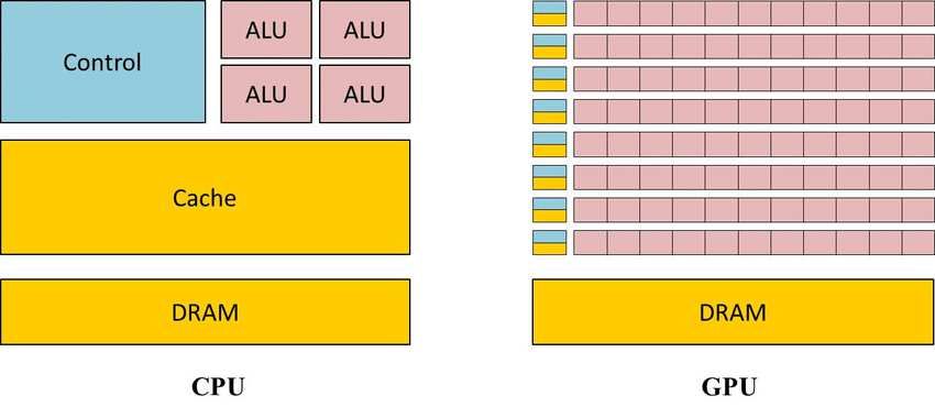
Figure 1: GPU architecture.
Airy function are defined as
∞ m
(−1) x
Jα (x) = ( )2m+α in such a way that it uses GPU architecture efficiently. In fact,
m!Γ(m + α + 1) 2
m=0 acceleration is provided by data parallel processing for the
2
algorithms which are present outside the field of rendering
( x4 )k
∞
x and processing of image. The GPU used in order to carry out
Iα (x) = ( )α the work represented in this paper is NVIDIA Tesla K80.
2 k!Γ(k + α + 1)
k=0
π I−α (x) − Iα (x) Specifications of NVIDIA Tesla K80 GPU
Kα (x) =
2 sin(απ) The following are the GPU device specifications used
during computing and evaluating the Airy function.
Here Γ(x) is the Gamma Function. The Bessel functions have
there applications in Fluid dynamics, Electrodynamics and
mainly in Acoustics [25]. Table I: NVIDIA Tesla K80 GPU specifications.
Parameters Specifications
III. G RAPHICS P ROCESSING U NIT (GPU) Peak Double Precision Floating point precision 2.91 Tflops
Peak Single Precision Floating point precision 8.74 Tflops
Graphic rendering is all about compute intensiveness and Memory Bandwidth(ECC Off) 480GB/sec
highly parallel computation. These are the features or special- Memory size and Type 24GB GDDR5
ization of Graphic Processor unit or GPU [6]. The process of CUDA corecores 4992
Thermal solution Passive heat sink
generation of an image from a 2D or 3D model by means of
computer programs is called rendering. This process needs a
huge number of calculations to be performed in fraction of
seconds. GPU has developed gradually into a highly parallel Computation of GPU using MATLAB
and multi threaded processor which consists of many cores.
The computational horsepower of GPU is enormous and also The Matrix Laboratory, MATLAB is a programming plat-
it has high memory bandwidth. The floating point capability of form constructed especially for engineers and scientists. It
GPU and CPU has inconsistency between them. Not only this makes use of the MATLAB language, a matrix based language,
but there are also differences between the architecture of GPU granting the most logical expression of computational math-
and traditional CPU. The CPU provides more resources to ematics. MATLAB is used by millions of engineers world-
make single instruction execute faster, whereas the GPU makes wide. The reason behind its usage is to analyse and design
use of hundreds of individual processing elements (cores) to the systems and products for revolutionizing our world. As
execute single instruction on multiple data elements (elements MATLAB’s operation is on whole matrices and arrays, it is one
in array) in parallel [2]. It is designed in such a way that of the efficient ways to express computational mathematics.
more transistors are devoted to data processing rather than data For envision and to obtain the insights from data, built in
caching and flow control. graphics are utilised which furthermore makes it an easy
job. The desktop environment (DE) gives an opportunity to
To get a speedup in computation time, the applications experiment, analyse and discover. These tools of MATLAB and
consisting of large data sets make use of the platform of its effectiveness are all precisely tested and constructed to work
data parallel programming, the applications of processing of together [7]. Parallel Computing Toolbox present in MATLAB
image and media which includes the post-process of image lets one to solve computationally and data-intensive problems
synthesis, video encoding and decoding, resizing of a digital using multi core processors like GPUs. Some of the High level
image, stereo vision and automated recognition of patterns and constructs like parallel for loops and parallelized numerical
regularities in data which maps the image blocks and pixels to algorithms enables us to parallelize MATLAB applications.
parallel processing threads.It is quite obvious that a GPU will The toolbox allows one to use the full processing power
take less time for computing as compared to CPU, but the catch of multi core desktops by executing applications on workers
is to write a program by utilising special function/subroutines that run locally [8]. The Parallel Computing Toolbox (PCT)
3ITM Web of Conferences 32, 03052 (2020) https://doi.org/10.1051/itmconf/20203203052
ICACC-2020
requires the NVIDIA CUDA enabled device with compute 5) Compare the output thus obtained with that of MAT-
capability of 1.3 or greater [2]. LAB’s result.
6) If the answer is not of the desired precision, make
IV. D ESIGN O F IMPLEMENTATION the necessary changes in the code.
7) Prepare a vectorized code for the same (for GPU).
Some of the functions used while computing in GPU are 8) Dump the code in GPU and thus calculate the time
as follows: required for implementation.
• gpuArray: This function is used to transfer the input 9) On calculating the time required for the same code
data from MATLAB workspace to GPU. This function in CPU, obtain the Speedup parameter by using the
converts the array in the MATLAB workspace into a following formula:
gpuArray object [8]. CP U T ime(Tc )
Speedup = (13)
• gather: For transferring the data from GPU to MAT- GP U T ime(Tg )
LAB workspace this function is used. The gather
function is used after all the operations on the data 10) Compile and analyse the results.
are performed by GPU.
The Airy function is implemented on CPU and similarly on
• gpuDevice: For displaying the properties of the cur- GPU by following the steps given in the above algorithm. Vec-
rently selected GPU device, the command gpuDevice torization of code is important while implementing the function
is used. in GPU because it eliminates loops which are sequentially
executed. All the operations performed on the data transferred
Following are the steps to be followed while running a
to GPU memory are executed on GPU in parallel by using
MATLAB code on GPU:
MATLAB’s PCT. The above algorithm can be generalized for
1) Start with the correct code which gives appropriate any function.
results.
2) Perform Vectorization of the code.
3) Profile the code using Run and Time function. V. R ESULTS AND A NALYSIS
4) Variables should be transferred to GPU memory using In this section a rigorous comparative study of computation
gpuArray() function. time required for evaluating the Airy function on NVIDIA
5) After the execution of code is done the output vari- Tesla K80 CPU and GPU is presented. It should be taken into
ables must be transferred to CPU memory by using account that both functions (Airy function of first kind and
gather() function. second kind) were evaluated on total 9 test input in ascending
The definitions of Airy function used while implementing order as shown in table 2 and 3 for 10000 times on CPU as
it are as follows: well as GPU, and the computational time was noted down
for both platforms. After that a mean was calculated for each
input and listed in tables below. The reason behind doing so
Ai(x) = is to eliminate any statistical anomaly or error that might have
� 3 3 occurred unknowingly while calculating the computation time.
x
(J 1 ( 2 x 2 ) + J− 13 ( 32 x 2 )) ,x < 0 At last the Speedup parameter is calculated by the formula
29 3 3
33
,x = 0 given in the algorithm described in section 4.
Γ( 32 )
1 2 32
�x
3K3 (3x ) ,x > 0
π
1 The following two tables present the computational time
and the Speedup parameter for the purpose as discussed above.
The table 2 is for Ai(x) and table 3 is for Bi(x). We can infer
from table 2 that for Ai(x) the Speedup parameter calculated
using the device used in this experiment gives an improvement
Bi(x) = in computation time (for largest input) of around 2.667 times
�
x 2 32 2 32 the computation time required for the CPU to evaluate the same
3 (J 3 ( 3 x ) − J− 3 ( 3 x )) ,x < 0
1 1
function with the same input on GPU. This is the crux of using
−1
3 6 GPUs multi-core architecture instead of single or dual core
Γ( 32 )
,x = 0
� x (I 1 ( 2 x 32 ) + I 1 ( 2 x 23 ))
CPUs. Similarly for Bi(x) the table 3 shows that the calculated
3 3 3 −3 3 ,x > 0 Speedup parameter is around 2.601 for the same system as
The following algorithm represents steps of implementation of mentioned above. The Speedup parameter depends on various
Airy function: factors that can decrease its value. As mentioned in section 2,
for every function a different subroutine was used to evaluate
1) Start with the definition of Airy function used. the code, because of the complexity of the Airy function it
2) Write a pseudo-code for the function on paper. calculates a total of 5 subroutines to evaluate the final Ai(x) or
3) Write the actual code for the function in MATLAB Bi(x) value. The function was not hardcoded (implementing
and obtain the output. Bessel and Airy functions into one single subroutine) as in
4) Do the calculations of Airy function using Bessel real world application where this function might be used there
function manually. would be an existing definition of the Bessel function.
4ITM Web of Conferences 32, 03052 (2020) https://doi.org/10.1051/itmconf/20203203052
ICACC-2020
[10] “Parallel Computing”, Wolfram Mathworld. [Online]. Available:
Table II: Speedup parameter for Airy function of first kind. http://mathworld.wolfram.com/ParallelComputing.html
Argument for Ai(x) CPU Time (Tc in ms) GPU Time (Tg in ms) Speedup
[11] “Best Practices for MATLAB GPU Coding”, Cornell
1 0.494 0.186 2.655913978 University Center for Advanced Computing. [Online]. Available:
2 0.475 0.184 2.581521739
https://www.cac.cornell.edu/matlab
3 0.474 0.183 2.590163934
4 0.473 0.182 2.598901099 [12] Ç. Uluişik and L. Sevgi, “A Tutorial on Bessel Functions and Numerical
5 0.473 0.181 2.613259669 Evaluation of Bessel Integrals,” in IEEE Antennas and Propagation
10 0.467 0.181 2.580110497 Magazine, vol. 51, no. 6, pp. 222-233, Dec. 2009.
50 0.455 0.177 2.570621469 [13] Amparo Gil , Javier Segura , Nico M.Temme,“Numerical methods for
100 0.447 0.174 2.568965517
special functions-Society for industrial and Applied Mathematics”.
1000 0.448 0.168 2.666666667
[14] B.K.Agarwal, Hari Prakash 2016,Quantum Mechanics,PHI,Delhi.
[15] A. K. Ghatak, R. L. Gallawa and I. C. Goyal,“Accurate solutions to
Schrodinger’s equation using modified Airy function,” in IEEE Journal
of Quantum Electronics, vol. 28, no. 2, pp. 400-403, Feb. 1992.
Table III: Speedup parameter for Airy function of Second kind. [16] B. Zhang, S. Xu, F. Zhang, Y. Bi and L. Huang ,“Accelerating MATLAB
Argument for Bi(x) CPU Time (Tc in ms) GPU Time (Tg in ms) Speedup code using GPU:A review of tools and strategies”. Artificial Intelligence,
1 0.468 0.191 2.450261783 Management Science and ElectronicCommerce(AIMSEC):Dengleng,
2 0.463 0.190 2.436842105 China, Aug. 2011.
3 0.461 0.189 2.439153439 [17] Fractional-order modeling of neutron transport in a nuclear reactor , by
4 0.460 0.185 2.486486486 Vishwesh A.Vyawahare, P.S.V.Nataraj.
5 0.457 0.184 2.483695652
10 0.453 0.180 2.516666667 [18] G. Chen, G. Li, S. Pei and B. Wu, “High Performance Computing via
50 0.450 0.176 2.556818182 a GPU” 2009 First International Conference on Information Science and
100 0.447 0.173 2.583815029 Engineering, Nanjing, 2009, pp. 238-241.
1000 0.437 0.168 2.601190476 [19] P. Sebah and X. Gourdon,“Introduction to the gamma function”, Amer-
ican Journal of Scientific Research, Feb. 2002.
[20] D. W. Lozier, “NIST digital library of mathematical functions”, Annals
of Mathematics and Artificial Intelligence, Springer, May 2003.[Online].
VI. C ONCLUSION Available:https://link.springer.com/article/
The work which was carried out was the acceleration of [21] E. Lindholm, J. Nickolls, S. Oberman and J. Montrym, “NVIDIA Tesla:
computation of Airy function on GPU. The acceleration is A Unified Graphics and Computing Architecture,” in IEEE Micro, vol.
28, no. 2, pp. 39-55, March-April 2008.
obtained because of the presence of multiple processing cores
[22] Abramowitz, Milton; Stegun, Irene Ann, eds. (1983) [June 1964].
in GPU. A validation for the function was set using MATLAB. ”Chapter 10”. Handbook of Mathematical Functions with Formulas,
The same code was transformed into vectorized version using Graphs, and Mathematical Tables. Applied Mathematics Series. 55
Parallel Computing toolbox of MATLAB. From the results, (Ninth reprint with additional corrections of tenth original printing with
it is observed that the computational time required for the corrections (December 1972); first ed.). Washington D.C.; New York:
execution is more in CPU as compared to GPU. Thus the United States Department of Commerce, National Bureau of Standards;
Dover Publications. p. 446. ISBN 978-0-486-61272-0. LCCN 64-60036.
Speedup parameter obtained is around 2 to 3 fold for Airy MR 0167642. LCCN 65-12253.
function when evaluated on systems with NVIDIA Tesla K80 [23] Digital Library of Mathematical Functions, National Institute of Stan-
GPU. From the results it may be concluded that Speedup dards and Technology, available at http://dlmf.nist.gov/.
parameter depends on the amount of data and number of [24] Donald A. Neamen,“Semiconductor Physics and Devices”,chapter 2 -
iterations of an operation. Introduction to Quantum theory of solids .
[25] K. Parand, M. Nikarya,Application of Bessel functions for solving dif-
R EFERENCES ferential and integro-differential equations of the fractional order,Applied
Mathematical Modelling,Volume 38, Issues 15–16,2014,Pages 4137-
[1] V. Kiryakova, “The special functions of fractional calculus as generalized 4147,ISSN 0307-904X,https://doi.org/10.1016/j.apm.2014.02.001.
fractional calculus operators of some basic functions,” Computers and [26] Katugampola, Udita N. (15 October 2014). ”A New Approach To
Mathematics with Applications, vol. 59, no. 3, pp. 1128-1141, Feb. 2010 Generalized Fractional Derivatives” (PDF). Bulletin of Mathemati-
[2] Patil Parag,Singhaniya Navin,Jage Chaitanya,Vyawahare Vishwesh,Patil cal Analysis and Applications. 6 (4): 1–15. arXiv:1106.0965. Bib-
Mukesh and Paluri Nataraj. (2018). GPU Computing of code:2011arXiv1106.0965K.
Special Mathematical Functions used in Fractional Calculus. [27] Niels Henrik Abel (1823). ”Oplösning af et par opgaver ved hjelp af
10.2174/9781681085999118010011. bestemte integraler (Solution de quelques problèmes à l’aide d’intégrales
[3] Olivier Vallee and Manuel Soares - Airy function and applications in définies, Solution of a couple of problems by means of definite integrals)”
physics (PDF). Magazin for Naturvidenskaberne. Kristiania (Oslo): 55–68.
[4] J. Liu, C. Gong, W. Bao, G. Tang, and Y. Jiang, “Solving the Caputo [28] Tenreiro Machado, José Kiryakova, Virginia Mainardi, Francesco.
fractional reactiondiffusion equation on GPU”, Discrete Dynamics in (2011). Recent history of fractional calculus. Communications in Nonlin-
Nature and Society, Hindawi Publishing Corporation, vol. 2014, 2014. ear Science and Numerical Simulation - COMMUN NONLINEAR SCI
[5] N. E. Banks, “Insights from the parallel implementation of efficient NUMER SI. 16. 1140-1153. 10.1016/j.cnsns.2010.05.027.
algorithms for the fractional calculus”, University of Chester, United [29] Kreyszig, Erwin. Advanced Engineering Mathematics. New York :Wi-
Kingdom, 2015 ley, 1983.
[6] Nvidia, CUDA C Programming Guide , Ver. 7.5, Sep. 2015. [Online]. [30] NVIDIA. (2015). TESLA K80 GPU ACCELERATOR - Board speci-
Available: https://developer.nvidia.com/hpc fications [PDF file]. Available: https://www.nvidia.com/content/dam/en-
[7] “MATLAB Documentation” https://in.mathworks.com/help/matlab/ zz/Solutions/Data-Center/tesla-product-literature/Tesla-K80-BoardSpec-
07317-001-v05.pdf
[8] Available:https://in.mathworks.com/help/parallel-
computing/index.html’stid=CRUXlftnav
[9] “Predicting and Measuring Parallel Performance”, February 1, 2012.
[Online]. Available:https://software.intel.com
5You can also read