Incorporating Interpretable Output Constraints in Bayesian Neural Networks - Finale Doshi-Velez
←
→
Page content transcription
If your browser does not render page correctly, please read the page content below
Incorporating Interpretable Output Constraints
                                                         in Bayesian Neural Networks

                                                   Wanqian Yang                          Lars Lorch∗                   Moritz A. Graule
                                                 Harvard University                      ETH Zürich                    Harvard University
                                                Cambridge, MA, USA                 8092 Zürich, Switzerland           Cambridge, MA, USA
                                            yangw@college.harvard.edu             llorch@student.ethz.ch            graulem@g.harvard.edu
arXiv:2010.10969v2 [cs.LG] 6 Jan 2021

                                                         Himabindu Lakkaraju                                Finale Doshi-Velez
                                                           Harvard University                               Harvard University
                                                          Cambridge, MA, USA                               Cambridge, MA, USA
                                                     hlakkaraju@seas.harvard.edu                        finale@seas.harvard.edu

                                                                                        Abstract
                                                    Domains where supervised models are deployed often come with task-specific con-
                                                    straints, such as prior expert knowledge on the ground-truth function, or desiderata
                                                    like safety and fairness. We introduce a novel probabilistic framework for rea-
                                                    soning with such constraints and formulate a prior that enables us to effectively
                                                    incorporate them into Bayesian neural networks (BNNs), including a variant that
                                                    can be amortized over tasks. The resulting Output-Constrained BNN (OC-BNN) is
                                                    fully consistent with the Bayesian framework for uncertainty quantification and is
                                                    amenable to black-box inference. Unlike typical BNN inference in uninterpretable
                                                    parameter space, OC-BNNs widen the range of functional knowledge that can be
                                                    incorporated, especially for model users without expertise in machine learning. We
                                                    demonstrate the efficacy of OC-BNNs on real-world datasets, spanning multiple
                                                    domains such as healthcare, criminal justice, and credit scoring.

                                        1        Introduction
                                        In domains where predictive errors are prohibitively costly, we desire models that can both capture
                                        predictive uncertainty (to inform downstream decision-making) as well as enforce prior human
                                        expertise or knowledge (to induce appropriate model biases). Performing Bayesian inference on deep
                                        neural networks, which are universal approximators [11] with substantial model capacity, results in
                                        BNNs — models that combine high representation power with quantifiable uncertainty estimates
                                        [21, 20] 1 . The ability to encode informative functional beliefs in BNN priors can significantly
                                        reduce the bias and uncertainty of the posterior predictive, especially in regions of input space
                                        sparsely covered by training data [27]. Unfortunately, the trade-off for their versatility is that BNN
                                        priors, defined in high-dimensional parameter space, are uninterpretable. A general approach for
                                        incorporating functional knowledge (that human experts might possess) is therefore intractable.
                                        Recent work has addressed the challenge of incorporating richer functional knowledge into BNNs,
                                        such as preventing miscalibrated model predictions out-of-distribution [9], enforcing smoothness
                                        constraints [2] or specifying priors induced by covariance structures in the dataset (cf. Gaussian
                                        processes) [25, 19]. In this paper 2 , we take a different direction by tackling functional knowledge
                                        expressed as output constraints — the set of values y is constrained to hold for any given x. Unlike
                                        other types of functional beliefs, output constraints are intuitive, interpretable and easily specified,
                                            ∗
                                               Work done while at Harvard University.
                                             1
                                               See Appendix A for a technical overview of BNN inference and acronyms used throughout this paper.
                                             2
                                               Our code is publicly available at: https://github.com/dtak/ocbnn-public.

                                        34th Conference on Neural Information Processing Systems (NeurIPS 2020), Vancouver, Canada.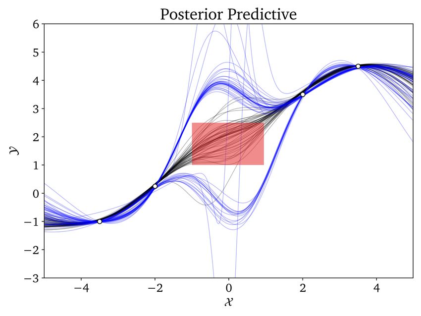
even by domain experts without technical understanding of machine learning methods. Examples
include ground-truth human expertise (e.g. known input-output relationship, expressed as scientific
formulae or clinical rules) or critical desiderata that the model should enforce (e.g. output should be
restricted to the permissible set of safe or fair actions for any given input scenario).
We propose a sampling-based prior that assigns probability mass to BNN parameters based on how
well the BNN output obeys constraints on drawn samples. The resulting Output-Constrained BNN
(OC-BNN) allows the user to specify any constraint directly in its functional form, and is amenable
to all black-box BNN inference algorithms since the prior is ultimately evaluated in parameter space.
Our contributions are: (a) we present a formal framework that lays out what it means to learn from
output constraints in the probabilistic setting that BNNs operate in, (b) we formulate a prior that
enforces output constraint satisfaction on the resulting posterior predictive, including a variant that
can be amortized across multiple tasks, (c) we demonstrate proof-of-concepts on toy simulations
and apply OC-BNNs to three real-world, high-dimensional datasets: (i) enforcing physiologically
feasible interventions on a clinical action prediction task, (ii) enforcing a racial fairness constraint on
a recidivism prediction task where the training data is biased, and (iii) enforcing recourse on a credit
scoring task where a subpopulation is poorly represented by data.

2   Related Work
Noise Contrastive Priors Hafner et al. [9] propose a generative “data prior” in function space,
modeled as zero-mean Gaussians if the input is out-of-distribution. Noise contrastive priors are
similar to OC-BNNs as both methods involve placing a prior on function space but performing
inference in parameter space. However, OC-BNNs model output constraints, which encode a richer
class of functional beliefs than the simpler Gaussian assumptions encoded by NCPs.
Global functional properties Previous work have enforced various functional properties such as
Lipschitz smoothness [2] or monotonicity [29]. The constraints that they consider are different from
output constraints, which can be defined for local regions in the input space. Furthermore, these
works focus on classical NNs rather than BNNs.
Tractable approximations of stochastic process inference Garnelo et al. [7] introduce neural
processes (NP), where NNs are trained on sequences of input-output tuples {(x, y)i }m         i=1 to learn
distributions over functions. Louizos et al. [19] introduce a NP variant that models the correlation
structure of inputs as dependency graphs. Sun et al. [25] define the BNN variational objective directly
over stochastic processes. Compared to OC-BNNs, these models represent a distinct direction of
work, since (i) VI is carried out directly over function-space terms, and (ii) the set of prior functional
assumptions is different; they cannot encode output constraints of the form that OC-BNNs consider.
Equality/Inequality constraints for deep probabilistic models Closest to our work is that of
Lorenzi and Filippone [18], which incorporates equality and inequality constraints, specified as
differential equations, into regression tasks. Similar to OC-BNNs, constraint (C) satisfaction is
modeled as the conditional p(Y, C|x), e.g. Gaussian or logistic. However, we (i) consider a broader
framework for reasoning with constraints, allowing for diverse constraint formulations and defined for
both regression and classification tasks, and (ii) verify the tractability and accuracy of our approach
on a comprehensive suite of experiments, in particular, high-dimensional tasks.

3   Notation
Let X ∈ X where X = RQ be the input variable and Y ∈ Y be the output variable. For regression
tasks, Y = R. For K-classification tasks, Y is any set with a bijection to {0, 1, . . . , K − 1}. We
denote the ground-truth mapping (if it exists) as f ∗ : X → Y. While f ∗ is unknown, we have access
to observed data Dtr = {xi , yi }Ni=1 , which may be noisy or biased. A conventional BNN is denoted
as ΦW : X → Y. W ∈ W, where W = RM , are the BNN parameters (weights and biases of all
layers) represented as a flattened vector. All BNNs that we consider are multilayer perceptrons with
RBF activations. Uppercase notation denotes random variables; lowercase notation denotes instances.

4   Output-Constrained Priors
In joint X × Y space, our goal is to constrain the output y for any set of inputs x. In this setting,
classical notions of “equality” and “inequality” (in constrained optimization) respectively become
positive constraints and negative constraints, specifying what values y can or cannot take.

                                                    2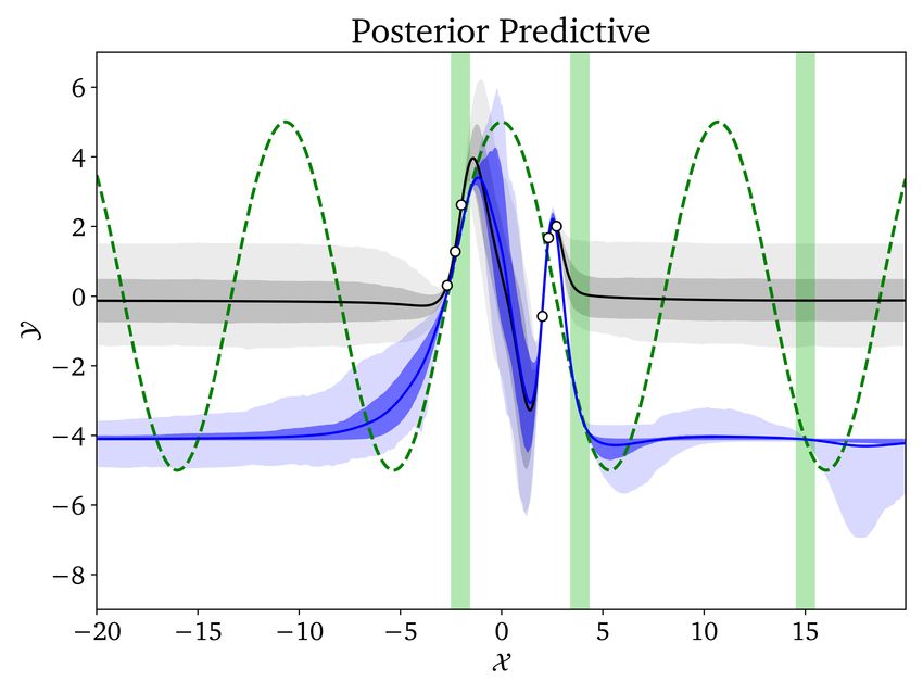
Definition 4.1. A deterministic output constraint C is a tuple (Cx , Cy , ◦) where Cx ⊆ X , Cy : Cx →
2Y and ◦ ∈ {∈, ∈}. / C is satisfied by an output y iff ∀ x ∈ Cx , y ◦ Cy (x). C + := C is a positive
constraint if ◦ is ∈. C − := C is a negative constraint if ◦ is ∈.
                                                                / C is a global constraint if Cx = X .
C is a local constraint if Cx ⊂ X .
The distinction between positive and negative constraints is not trivial because the user typically
has access to only one of the two forms. Positive constraints also tend to be more informative than
negative constraints. Definition 4.1 alone is not sufficient as we must define what it means for a BNN,
which learns a predictive distribution, to satisfy a constraint C. A natural approach is to evaluate the
probability mass of the prior predictive that satisfies a constraint.
Definition 4.2. A deterministic output constraint C = (Cx , Cy , ◦) is -satisfied by a BNN with prior
W ∼ p(w) if, ∀ x ∈ Cx and for some  ∈ [0, 1]:
                          Z
                              I[y ◦ Cy (x)] · p(ΦW = y|x) dy ≥ 1 −                                (1)
                                   Y
                       R
where p(ΦW |x) :=          W
                               p(Φw (x)|x, w) p(w) dw is the BNN prior predictive.
The strictness parameter  can be related to hard and soft constraints in optimization literature; the
constraint is hard iff  = 0. Note that  is not a parameter of our prior, instead, (1) is the goal
of inference and can be empirically evaluated on a test set. Since BNNs are probabilistic, we can
generalize Definition 4.1 further and specify a constraint directly as some distribution over Y :
Definition 4.3. A probabilistic output constraint C is a tuple (Cx , Dy ) where Cx ⊆ X and Dy (x) is
a distribution over Y. (That is, Dy , like Cy , is a partial function well-defined on Cx .) C is -satisfied
by a BNN with prior W ∼ p(w) if, ∀ x ∈ Cx and for some  ∈ [0, 1]:

                                 DDIV p(ΦW |x) Dy (x)                 ≤                                 (2)

where DDIV is any valid measure of divergence between two distributions over Y.
We seek to construct a prior W ∼ p(w) such that the BNN -satisfies, for some small , a specified
constraint C. An intuitive way to connect a prior in parameter space to C (defined in function space)
is to evaluate how well the implicit distribution of ΦW , induced by the distribution of W, satisfies C.
In Section 4.1, we construct a prior that is conditioned on C and explicitly factors in the likelihood
p(C|w) of constraint satisfaction. In Section 4.3, we present an amortized variant by performing
variational optimization on objectives (1) or (2) directly.
4.1 Conditional Output-Constrained Prior
A fully Bayesian approach requires a proper distribution that describes how well any w ∈ W satisfies
C by way of Φw . Informally, this distribution must be conditioned on all x ∈ Cx (though we sample
finitely during inference) and is the “product” of how well Φw (x) satisfies C for each x ∈ Cx . This
notion can be formalized by defining C as a stochastic process indexed on Cx .
Let x ∈ Cx be any single input. In measure-theoretic terms, the corresponding output Y : Ω → Y is
defined on some probability space (Ω, F, Pg,x ), where Ω and F are the typical sample space and
σ-algebra, and Pg,x is any valid probability measure corresponding   Q          to a distribution pg (·|x) over Y.
Then (Ω, F, Pg ) is the joint probability space, where Ω = x∈Cx Ω, F is the product σ-algebra and
Pg = x∈Cx Pg,x is the product measure (a pushforward measure from Pg,x ). Let CP : Ω → Y Cx
       Q

be the stochastic process indexed by Cx , where Y Cx denotes the set of all measurable functions from
Cx into Y. The law of the process CP is p(S) = Pg ◦ CP −1 (S) for all S ∈ Y Sx . For any finite
subset {Y (1) , . . . , Y (T ) } ⊆ CP indexed by {x(1) , . . . , x(T ) } ⊆ Cx ,
                                                                     T
                                                                     Y
                     p(Y (1) = y (1) , . . . , Y (T ) = y (T ) ) =         pg (Y (t) = y (t) |x(t) )          (3)
                                                                     t=1

CP is a valid stochastic process as it satisfies both (finite) exchangeability and consistency, which are
sufficient conditions via the Kolmogorov Extension Theorem [23]. As the BNN output Φw (x) can
be evaluated for all x ∈ Cx and w ∈ W, CP allows us to formally describe how much Φw satisfies
C, by determining the measure of the realization ΦCwx ∈ Y Cx .

                                                          3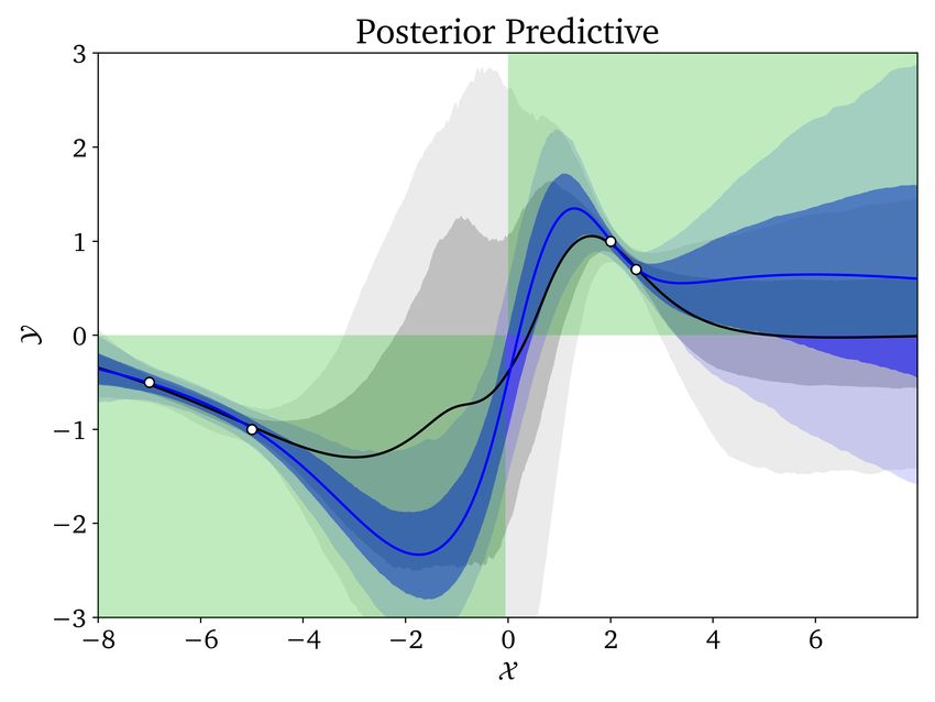
Definition 4.4. Let C be any (deterministic or probabilistic) constraint and CP the the stochastic
process defined on Y Cx for some measure Pg . The conditional output-constrained prior (COCP)
on W is defined as
                                     pC (w) = pf (w)p(ΦCwx )                                   (4)
                                                                      Cx     Cx
where pf (w) is any distribution on W that is independent of C, and Φw ∈ Y is the realization of
CP corresponding to the BNN output Φw (x) for all x ∈ Cx .
We can view (4) loosely as an application of Bayes’ Rule, where the realization ΦCwx of the stochastic
process CP is the evidence (likelihood) of C being satisfied by w and pf (w) is the unconditional
prior over W. This implies that the posterior that we are ultimately inferring is W|Dtr , CP, i.e. with
extra conditioning on CP. To ease the burden on notation, we will drop the explicit conditioning on
CP and treat pC (w) as the unconditional prior over W. To make clear the presence of C, we will
denote the constrained posterior as pC (w|Dtr ). Definition 4.4 generalizes to multiple constraints
C (1) , . . . , C (m) by conditioning on all C (i) and evaluating Φw for each constraint. Assuming the
                                                                       Qm        C (i)
constraints to be mutually independent, pC (1) ,...,C (m) (w) = pf (w) i=1 p(Φwx ).
It remains to describe what measure Pg we should choose such that p(ΦCwx ) is a likelihood distribution
that faithfully evaluates the extent to which C is satisfied. For probabilistic output constraints, we
simply set pg (·|x) to be Dy (x). For deterministic output constraints, we propose a number of
distributions over Y that corresponds well to Cy , the set of permitted (or excluded) output values.
Example: Positive Mixture of Gaussian Constraint A positive constraint C + for regression,
where Cy (x) = {y1 , . . . , yK } contains multiple values, corresponds to the situation wherein the
expert knows potential ground-truth values over Cx . A natural choice is the Gaussian mixture model:
          PK
CP(x) ∼ k=1 ωk N (yk , σC2 ), where σC is the standard deviation of the Gaussian, a hyperparameter
                                                                             PK
controlling the strictness of C satisfaction, and ωk are the mixing weights: k=1 ωk = 1.
Example: Positive Dirichlet Constraint For K-classification, the natural distribution to consider
is the Dirichlet distribution, whose support (the standard K-simplex) corresponds to the K-tuple of
predicted probabilities on all classes. For a positive constraint C + , we specify:

                                         γ           if i ∈ Cy (x)
       CP(x) ∼ Dir(α);           αi =                                    where γ ≥ 1, 0 < c < 1 (5)
                                         γ(1 − c) otherwise

Example: Negative Exponential Constraint A negative constraint C − for regression takes Cy (x)
to be the set of values that cannot be the output of x. For the case where Cy is determined from
a set of inequalities of the form {g1 (x, y) ≤ 0, . . . , gl (x, y) ≤ 0}, where obeying all inequalities
implies that y ∈ Cy (x) and hence C − is not satisfied, we can consider an exponential distribution that
penalizes y based on how each inequality is violated:
                                                  n          l
                                                             Y                              o
                      pg (CP(x) = y 0 |x) ∝ exp       −γ·          στ0 ,τ1 (gi (x, y 0 ))            (6)
                                                             i=1

where στ0 ,τ1 (z) = 14 (tanh(−τ0 z) + 1)(tanh(−τ1 z) + 1) and γ is a decay hyperparameter. The
sigmoidal function στ0 ,τ1 (gi (x, y 0 )) is a soft indicator of whether gi ≤ 0 is satisfied. pg (CP(x) =
y 0 |x) is small if every gi (x, y 0 ) ≤ 0, i.e. all inequalities are obeyed and C − is violated.
4.2 Inference with COCPs
A complete specification of (4) is sufficient for inference using COCPs, as the expression pC (w) can
simply be substituted for that of p(w) in all black-box BNN inference algorithms. Since (4) cannot
be computed exactly due to the intractability of p(ΦCwx ) for uncountable Cx , we will draw a finite
sample {x(t) }Tt=1 of x ∈ Cx (e.g. uniformly across Cx or Brownian sampling if Cx is unbounded) at
the start of the inference process and compute (3) as an estimator of p(ΦCwx ) instead:
                                                  T
                                                  Y
                               p̃C (w) = pf (w)         pg (Φw (x(t) )|x(t) )                        (7)
                                                  t=1
The computational runtime of COCPs increases with the input dimensionality Q and the size of Cx .
However, we note that many sampling techniques from statistical literature can be applied to COCPs
in lieu of naive uniform sampling. We use the isotropic Gaussian prior for pf (w).

                                                   4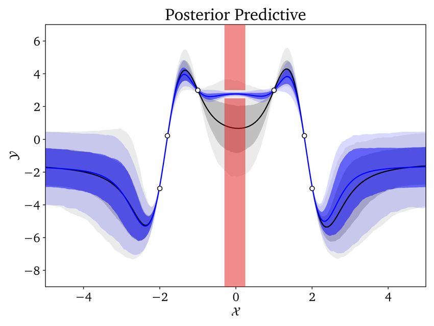
(a) Prior predictive plots.       (b) Posterior predictive plots.
Figure 1: 1D regression with the negative constraint: Cx− = [−0.3, 0.3] and Cy− = (−∞, 2.5]∪[3, ∞),
in red. The negative exponential COCP (6) is used. Even with such a restrictive constraint, the
predictive uncertainty of the OC-BNN (blue) drops sharply to fit within the permitted region of Y.
Note that the OC-BNN posterior uncertainty matches the baseline (gray) everywhere except near Cx .

Absolute guarantees of (1) or (2), i.e. achieving  = 0, are necessary in certain applications but
challenging for COCPs. Zero-variance or truncated pC (w), as means of ensuring hard constraint
satisfaction, are theoretically plausible but numerically unstable for BNN inference, particularly
gradient-based methods. Nevertheless, as modern inference algorithms produce finite approximations
of the true posterior, practical guarantees can be imposed, such as via further rejection sampling on
top of the constrained posterior pC (w|Dtr ). We demonstrate in Section 5 that unlike naive rejection
sampling from p(w|Dtr ), doing so from pC (w|Dtr ) is both tractable and practical for ensuring zero
constraint violations.
4.3 An Amortized Output-Constrained Prior
Instead of constructing a PDF over w explicitly dependent on Φw and C, we can learn a variational
approximation qλ (w) where we optimize λ directly with respect to our goals, (1) or (2). As both
objectives contain an intractable expectation over W, we seek a closed-form approximation of the
variational prior predictive pλ (ΦW |x). For the regression and binary classification settings, there
are well-known approximations, which we state in Appendix B as (17) and (21) respectively. Our
objectives are:                        Z
                         λ∗ = arg max      I[y ◦ Cy (x)] · pλ (ΦW = y|x) dy                       (8)
                                   λ∈Λ Y

                            λ∗ = arg min DDIV pλ (ΦW |x) Dy (x)                                   (9)
                                        λ∈Λ
As (8) and (9) are defined for a specific x ∈ Cx , we need to stochastically optimize over all x ∈ Cx .
Even though (8) is still an integral over Y, it is tractable since we only need to compute the CDF
corresponding to the boundary elements of Cy . We denote the resulting learnt distribution qλ∗ (w)
as the amortized output-constrained prior (AOCP). Unlike COCPs, where pC (w) is directly
evaluated during posterior inference, we first perform optimization to learn λ∗ , which can then be
used for inference independently over any number of training tasks (datasets) Dtr .

5   Low-Dimensional Simulations
COCPs and AOCPs are conceptually simple but work well, even on non-trivial output constraints. As
a proof-of-concept, we simulate toy data and constraints for small input dimension and visualize the
predictive distributions. See Appendix C for experimental details.
OC-BNNs model uncertainty in a manner that respects constrained regions and explains train-
ing data, without making overconfident predictions outside Cx . Figure 1 shows the prior and
posterior predictive plots for a negative constraint for regression, where a highly restrictive constraint
was intentionally chosen. Unlike the naive baseline BNN, the OC-BNN satisfies the constraint, with
its predictive variance smoothly narrowing as x approaches Cx so as to be entirely confined within
Y − Cy . After posterior inference, the OC-BNN fits all data points in Dtr closely while still respecting
the constraint. Far from Cx , the OC-BNN is not overconfident, maintaining a wide variance like the
baseline. Figure 2 shows an analogous example for classification. Similarly, the OC-BNN fits the
data and respects the constraint within Cx , without showing a strong preference for any class OOD.
OC-BNNs can capture global input-output relationships between X and Y, subject to sampling
efficacy. Figure 3a shows an example where we enforce the constraint xy ≥ 0. Even though the

                                                      5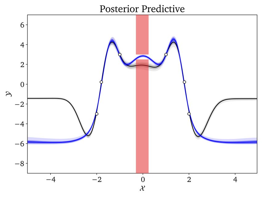
(a) Prior predictive plots.       (b) Posterior predictive plots.
Figure 2: 2D 3-classification with the positive constraint: Cx+ = (1, 3) × (−2, 0) and Cy+ = {green}.
The main plots are the OC-BNN predictives; insets are the baselines. Input region is shaded by the
predicted class if above a threshold certainty. The positive Dirichlet COCP (5) is used. In both the
prior and posterior, the constrained region (green rectangle) enforces the prediction of the green class.

      (a) Posterior predictive plots.    (b) Posterior predictive plots.         (c) Rejection sampling.
Figure 3: (a) 1D regression with the positive constraint: Cx+ = R and Cy+ (x) = {y | x · y ≥ 0}
(green), using AOCP. (b) 1D regression with the negative constraint: Cx− = [−1, 1] and Cy− = [1, 2.5]
(red), with the negative exponential COCP (6). The 50 SVGD particles represent functions passing
above and below the constrained region, capturing two distinct predictive modes. (c) Fraction of
rejected SVGD particles (out of 100) for the OC-BNN (blue, plotted as a function of log-samples
used with COCP) and the baseline (black). All baseline particles were rejected, however, only 4% of
particles were rejected, using just only 5 COCP samples.

training data itself adheres to this constraint, learning from Dtr alone is insufficient. The OC-BNN
posterior predictive narrows significantly (compared to the baseline) to fit the constraint, particularly
near x = 0. Note, however, that OC-BNNs can only learn as well as sampling from Cx permits.
OC-BNNs can capture posterior multimodality. As NNs are highly expressive, BNN posteriors
can contain multiple modes of significance. In Figure 3b, the negative constraint is specified in
such a way as to allow for functions that fit Dtr to pass both above or below the constrained region.
Accordingly, the resulting OC-BNN posterior predictive contains significant probability mass on
either side of Cy . Importantly, note that the negative exponential COCP does not explicitly indicate
the presence of multiple modes, showing that OC-BNNs naturally facilitate mode exploration.
OC-BNNs can model interpretable desiderata represented as output constraints. OC-BNNs
can be used to enforce important qualities that the system should possess. Figure 4 demonstrates a
fairness constraint known as demographic parity:
                                  p(Y = 1|xA = 1) = p(Y = 1|xA = 0)                                        (10)
where xA is a protected attribute such as race or gender. (10) is expressed as a probabilistic output
constraint. The OC-BNN not only learns to respect this constraint, it does so in the presence of
conflicting training data (Dtr is an unfair dataset).
Sensitivity to Inference and Conflicting Data Figure 5 in Appendix D shows the same negative
constraint used in Figure 1, except using different inference algorithms. There is little difference
in these predictive plots besides the idiosyncrasies unique to each algorithm. Hence OC-BNNs
behave reliably on, and are agnostic to, all major classes of BNN inference. If C and Dtr are
incompatible, such as with adversarial or biased data, the posterior depends on (i) model capacity
and (ii) factors affecting the prior and likelihood, e.g. volume of data or OC-BNN hyperparameters.
For example, Figure 6 in Appendix D shows a BNN with enough capacity to fit both the noisy data

                                                        6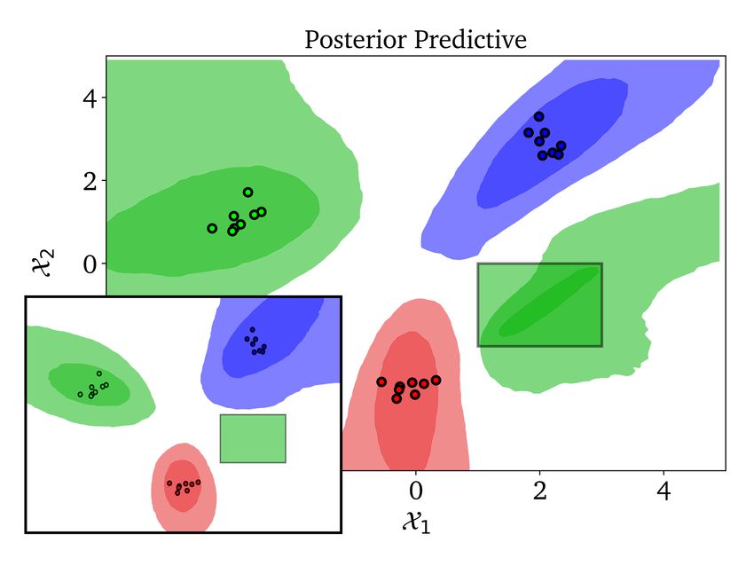
(a) Baseline posterior predictive. (b) OC-BNN posterior predictive.
Figure 4: 2D binary classification. Suppose a hiring task where X1 (binary) indicates membership of a
protected trait (e.g. gender or race) and X2 denotes skill level. Hence a positive (orange) classification
should be correlated with higher values of X2 . The dataset Dtr displays historic bias, where members
of the protected class (x1 = 1) are discriminated against (Y = 1 iff x1 = 1, x2 ≥ 0.8, but Y = 1 iff
x1 = 0, x2 ≥ 0.2). A naive BNN (a) would learn an unfair linear separator. However, learning the
probabilistic constraint: Dy (x) as the distribution where p(Φ(x) = 1) = x2 with the AOCP allows
the OC-BNN (b) to learn a fair separator, despite a biased dataset.

as well as ground-truth constraints, resulting in “overfitting” of the posterior predictive. However,
the earlier example in Figure 4 prioritizes the fairness constraint, as the small size of Dtr constitutes
weaker evidence.
Ensuring Hard Constraints using Rejection Sampling A few SVGD particles in Figure 3b
violate the constraint. While COCPs cannot guarantee  = 0 satisfaction, hard constraints can be
practically enforced. Consider the idealized, truncated predictive distributions of the baseline BNN
and OC-BNN, whereby for each x ∈ Cx , we set p(Y = y|x) = 0 where the constraint is violated
and normalize the remaining density to 1. These distributions represent zero constraint violation
(by definition) and can be obtained via rejection sampling from the baseline BNN or OC-BNN
posteriors. Figure 3c shows the results of performing such rejection sampling, using the same setup
as Figure 3b. As shown, rejection sampling is intractable for the baseline BNN (not a single SVGD
particle accepted), but works well on the OC-BNN, even when using only a small sample count from
Cx to compute pC (w). This experiment shows not only that naive rejection sampling (on ordinary
BNNs) to weed out posterior constraint violation is futile, but also that doing the same on OC-BNNs
is a practical workaround to ensure that hard constraints are satisfied, which is generally difficult to
achieve in ideal, probabilistic settings.

6     Experiments with Real-World Data
To demonstrate the efficacy of OC-BNNs, we apply meaningful and interpretable output constraints
on real-life datasets. As our method is the first such work for BNN classification, the baseline that we
compare our results to is an ordinary BNN with the isotropic Gaussian prior. Experimental details for
all three applications can be found in Appendix C.
6.1   Application: Clinical Action Prediction
                             Train                                     Test
                      Accuracy F1 Score           Accuracy      F1 Score Constraint Violation
        BNN            0.713       0.548           0.738         0.222          0.783
        OC-BNN         0.735       0.565           0.706         0.290          0.136
Table 1: Compared to the baseline, the OC-BNN maintains equally high accuracy and F1 score on
both train and test sets. The violation fraction decreased about six-fold when using OC-BNNs.

The MIMIC-III database [12] contains physiological features of intensive care unit patients. We
construct a dataset (N = 405K) of 8 relevant features and consider a binary classification task of
whether clinical interventions for hypotension management — namely, vasopressors or IV fluids —
should be taken for any patient. We specify two physiologically feasible, positive (deterministic)
constraints: (1) if the patient has high creatinine, high BUN and low urine, then action should be
taken (Cy = {1}); (2) if the patient has high lactate and low bicarbonate, action should also be
taken. The positive Dirichlet COCP (5) is used. In addition to accuracy and F1 score on the test

                                                     7
with race feature without race feature
BNN OC-BNN BNN OC-BNN
Accuracy 0.837 0.708 0.835 0.734
Train
F1 Score 0.611 0.424 0.590 0.274
African American High-Risk Fraction 0.355 0.335 0.309 0.203
Non-African American High-Risk Fraction 0.108 0.306 0.123 0.156
Table 2: The OC-BNN predicts both racial groups with almost equal rates of high-risk recidivism,
compared to a 3.5× difference on the baseline. However, accuracy metrics decrease (expectedly).
set (N = 69K), we also measure -satisfaction on the constraints as violation fraction, where we
sample 5K points in Cx and measure the fraction of those points violating either constraint.
Results Table 1 summarizes the experimental results. The main takeaway is that OC-BNNs
maintain classification accuracy while reducing constraint violations. The results show that OC-
BNNs match standard BNNs on all predictive accuracy metrics, while satisfying the constraints
to a far greater extent. This is because the constraints are intentionally specified in input regions
out-of-distribution, and hence incorporating this knowledge augments what the OC-BNN learns
from Dtr alone. This experiment affirms the low-dimensional simulations in Section 5, showing that
OC-BNNs are able to obey interpretable constraints without sacrificing predictive power.
6.2 Application: Recidivism Prediction
COMPAS is a proprietary model, used by the United States criminal justice system, that scores
criminal defendants on their risk of recidivism. A study by ProPublica in 2016 found it to be
racially biased against African American defendants [1, 16]. We use the same dataset as this study,
containing 9 features on N = 6172 defendants related to their criminal history and demographic
attributes. We consider the same binary classification task as in Slack et al. [24] — predicting whether
a defendant is profiled by COMPAS as being high-risk. We specify the fairness constraint that
the probability of predicting high-risk recidivism should not depend on race: for all (Cx = R9 )
individuals, the high-risk probability should be identical to their actual recidivism history (Dy is such
that p(y = 1) = two_year_recid). The AOCP is used. Dtr is incompatible with this constraint
since COMPAS itself demonstrates racial bias. We train on two versions of Dtr — with/without the
inclusion of race as an explicit feature. As the dataset is small and imbalanced, we directly evaluate
the training set. To measure -satisfaction, we report the fraction of the sensitive attribute (African
American defendants vs. non-African American defendants) predicted as high-risk recidivists.
Results Table 2 summarizes the results. By constraining recidivism prediction to the defendant’s
actual criminal history, OC-BNNs strictly enforce a fairness constraint. On both versions of
Dtr , the baseline BNN predicts unequal risk for the two groups since the output labels (COMPAS
decisions) are themselves biased. This inequality is more stark when the race feature is included, as
the model learns the explicit, positive correlation between race and the output label. For both datasets,
the fraction of the two groups being predicted as high-risk recidivists equalized after imposing the
constraint using OC-BNNs. Unlike the previous example, OC-BNNs have lower predictive accuracy
on Dtr than standard BNNs. This is expected since the training dataset is biased, and enforcing racial
fairness comes at the expense of correctly predicting biased labels.
6.3 Application: Credit Scoring Prediction
Young adults tend to be disadvantaged by credit scoring models as their lack of credit history results
in them being poorly represented by data (see e.g. [14]). We consider the Give Me Some Credit
dataset (N = 133K) [13], containing binary labels on whether individuals will experience impending
financial distress, along with 10 features related to demographics and financial history. Motivated by
Ustun et al. [26]’s work on recourse (defined as the extent that input features must be altered to change
the model’s outcome), we consider the feature RevolvingUtilizationOfUnsecuredLines
(RUUL), which has a ground-truth positive correlation with financial distress. We analyze how
much a young adult under 35 has to reduce RUUL to flip their prediction to negative in three cases: (i)
a BNN trained on the full dataset, (ii) a BNN trained on a blind dataset (age ≥ 35), (iii) an OC-BNN
with an actionability constraint: for young adults, predict “no financial distress” even if RUUL is
large. The positive Dirichlet COCP (5) is used. In addition to scoring accuracy and F1 score on
the entire test set (N = 10K); we measure the effort of recourse as the mean difference of RUUL
between the two outcomes (Ŷ = 0 or 1) on the subset of individuals where age < 35 (N = 1.5K).
8Results As can be seen in Table 3, the ground-truth positive correlation between RUUL and the
output is weak, and the effort of recourse is consequentially low. However, the baseline BNN naturally
learns a stronger correlation, resulting in a higher effort of recourse. This effect is amplified if the
BNN is trained on a limited dataset without data on young adults. When an actionability constraint is
enforced, the OC-BNN reduces the effort of recourse without sacrificing predictive accuracy on
the test set, reaching the closest to the ground-truth recourse.
Ground Truth BNN (Full) BNN (Blind) OC-BNN
Accuracy 0.890 0.871 0.895
Test
F1 Score 0.355 0.346 0.350
Effort of Recourse 0.287 0.419 0.529 0.379
Table 3: All three models have comparable accuracy on the test set. However, the OC-BNN has the
lowest recourse effort (closest to ground truth).
7 Discussion
The usage of OC-BNNs depends on how we view constraints in relation to data. The clinical
action prediction and credit scoring tasks are cases where the constraint is a complementary source
of information, being defined in input regions where Dtr is sparse. The recidivism prediction task
represents the paradigm where Dtr is inconsistent with the constraint, which serves to correct an
existing bias. Both approaches are fully consistent with the Bayesian framework, whereby coherent
inference decides how the likelihood and prior effects each shape the resulting posterior.
In contrast with [7, 19, 25], OC-BNNs take a sampling-based approach to bridge functional
and parametric objectives. The simplicity of this can be advantageous — output constraints are a
common currency of knowledge easily specified by domain experts, in contrast to more technical
forms such as stochastic process priors. While effective sampling is a prerequisite for accurate
inference, we note that the sampling complexity of OC-BNNs is tractable even at the dimensionality
we consider in Section 6. Note that we sample in X -space, which is much smaller than W-space.
OC-BNNs are intuitive to formulate and work well in real-life settings. Even though COCPs
and AOCPs echo well-known notions of data-based regularization, it is not immediately clear that
these ideas are effectual in practice, and lead to well-behaved posteriors with appropriate output
variance (both within and without constrained regions). Our work represents the first such effort (i) to
create a broad framework for reasoning with diverse forms of output constraints, and (ii) that solidly
demonstrates its utility on a corresponding range of real-life applications.
8 Conclusion
We propose OC-BNNs, which allow us to incorporate interpretable and intuitive prior knowledge, in
the form of output constraints, into BNNs. Through a series of low-dimensional simulations as well
as real-world applications with realistic constraints, we show that OC-BNNs generally maintain the
desirable properties of ordinary BNNs while satisfying specified constraints. OC-BNNs complement
a nascent strand of research that aims to incorporate rich and informative functional beliefs into deep
Bayesian models. Our work shows promise in various high-stakes domains, such as healthcare and
criminal justice, where both uncertainty quantification and prior expert constraints are necessary for
safe and desirable model behavior.
Broader Impact
Our work incorporates task-specific domain knowledge, in the form of output constraints, into BNNs.
We wish to highlight two key positive impacts. (1) OC-BNNs allow us to manipulate an interpretable
form of knowledge. They can be useful even to domain experts without technical machine learning
expertise, who can easily specify such constraints for model behavior. A tool like this can be used
alongside experts in the real world, such as physicians or judges. (2) Bayesian models like BNNs and
OC-BNNs are typically deployed in “high-stakes” domains, which include those with societal impact.
We intentionally showcase applications of high societal relevance, such as recidivism prediction
and credit scoring, where the ability to specify and satisfy constraints can lead to fairer and more
ethical model behavior.
9That being said, there are considerations and limitations. (1) If the model capacity is low (e.g.
the BNN is small), constraints and model capacity may interact in unexpected ways that are not
transparent to the domain expert. (2) Our sampling approach allows us to be very general in specifying
constraints, but it also creates a trade-off between computational efficiency and accuracy of constraint
enforcement. (3) Finally, the expert could mis-specify or even maliciously specify constraints. The
first two considerations can be mitigated by careful optimization and robustness checks; the latter by
making the constraints public and reviewable by others.
Acknowledgments and Disclosure of Funding
The authors are grateful to Srivatsan Srinivasan, Anirudh Suresh, Jiayu Yao and Melanie F. Pradier
for contributions to an initial version of this work [28], as well as Gerald Lim, M.B.B.S. for helpful
discussions on the clinical action prediction task. HL acknowledges support from Google. WY and
FDV acknowledge support from the Sloan Foundation.
References
[1] Julia Angwin, Jeff Larson, Surya Mattu, and Lauren Kirchner. Machine Bias: Risk Assessments
in Criminal Sentencing. ProPublica, 2016.
[2] Cem Anil, James Lucas, and Roger Grosse. Sorting Out Lipschitz Function Approximation. In
Proceedings of the 36th International Conference on Machine Learning, 2019.
[3] Christopher M Bishop. Pattern Recognition and Machine Learning. Springer, 2006.
[4] Charles Blundell, Julien Cornebise, Koray Kavukcuoglu, and Daan Wierstra. Weight Uncertainty
in Neural Networks. In Proceedings of the 32nd International Conference on Machine Learning,
2015.
[5] Simon Duane, Anthony D Kennedy, Brian J Pendleton, and Duncan Roweth. Hybrid Monte
Carlo. Physics Letters B, 195(2):216–222, 1987.
[6] John Duchi, Elad Hazan, and Yoram Singer. Adaptive Subgradient Methods for Online Learning
and Stochastic Optimization. Journal of Machine Learning Research, 12(Jul):2121–2159, 2011.
[7] Marta Garnelo, Jonathan Schwarz, Dan Rosenbaum, Fabio Viola, Danilo J Rezende, S.M. Ali
Eslami, and Yee Whye Teh. Neural Processes. In 35th ICML Workshop on Theoretical
Foundations and Applications of Deep Generative Models, 2018.
[8] Alex Graves. Practical Variational Inference for Neural Networks. In Advances in Neural
Information Processing Systems, pages 2348–2356, 2011.
[9] Danijar Hafner, Dustin Tran, Timothy Lillicrap, Alex Irpan, and James Davidson. Noise
Contrastive Priors for Functional Uncertainty. arXiv:1807.09289, 2018.
[10] Geoffrey E Hinton and Drew Van Camp. Keeping the Neural Networks Simple by Minimizing
the Description Length of the Weights. In Proceedings of the 6th Annual Conference on
Computational Learning Theory, pages 5–13, 1993.
[11] Kurt Hornik, Maxwell Stinchcombe, and Halbert White. Multilayer Feedforward Networks are
Universal Approximators. Neural Networks, 2(5):359–366, 1989.
[12] Alistair EW Johnson, Tom J Pollard, Lu Shen, H Lehman Li-wei, Mengling Feng, Mohammad
Ghassemi, Benjamin Moody, Peter Szolovits, Leo Anthony Celi, and Roger G Mark. MIMIC-III,
A Freely Accessible Critical Care Database. Scientific Data, 3:160035, 2016.
[13] Kaggle. Give Me Some Credit. http://www.kaggle.com/c/GiveMeSomeCredit/, 2011.
[14] Nathan Kallus and Angela Zhou. Residual Unfairness in Fair Machine Mearning from Prej-
udiced Data. In Proceedings of the 35th International Conference on Machine Learning,
2018.
[15] Diederik P Kingma and Max Welling. Auto-Encoding Variational Bayes. In Proceedings of the
2nd International Conference on Learning Representations, 2014.
10[16] Jeff Larson, Surya Mattu, Lauren Kirchner, and Julia Angwin. How We Analyzed the COMPAS
Recidivism Algorithm. ProPublica, 2016.
[17] Qiang Liu and Dilin Wang. Stein Variational Gradient Descent: A General Purpose Bayesian
Inference Algorithm. In Advances in Neural Information Processing Systems, pages 2378–2386,
2016.
[18] Marco Lorenzi and Maurizio Filippone. Constraining the Dynamics of Deep Probabilistic
Models. In Proceedings of the 35th International Conference on Machine Learning, 2018.
[19] Christos Louizos, Xiahan Shi, Klamer Schutte, and Max Welling. The Functional Neural
Process. In Advances in Neural Information Processing Systems, pages 8743–8754, 2019.
[20] David J C MacKay. Probable Networks and Plausible Predictions — a Review of Practical
Bayesian Methods for Supervised Neural Networks. Network: Computation in Neural Systems,
6(3):469–505, 1995.
[21] Radford M Neal. Bayesian Learning for Neural Networks. PhD thesis, University of Toronto,
1995.
[22] Radford M Neal. MCMC Using Hamiltonian Dynamics. Handbook of Markov Chain Monte
Carlo, 2(11):2, 2011.
[23] Bernt Øksendal. Stochastic Differential Equations. In Stochastic Differential Equations, pages
65–84. Springer, 2003.
[24] Dylan Slack, Sophie Hilgard, Emily Jia, Sameer Singh, and Himabindu Lakkaraju. Fooling
LIME and SHAP: Adversarial Attacks on Post hoc Explanation Methods. In Proceedings of the
3rd AAAI/ACM Conference on Artificial Intelligence, Ethics, and Society, pages 180–186, 2020.
[25] Shengyang Sun, Guodong Zhang, Jiaxin Shi, and Roger Grosse. Functional Variational
Bayesian Neural Networks. In Proceedings of the 7th International Conference on Learning
Representations, 2019.
[26] Berk Ustun, Alexander Spangher, and Yang Liu. Actionable Recourse in Linear Classification.
In Proceedings of the ACM Conference on Fairness, Accountability and Transparency, pages
10–19, 2019.
[27] Andrew Gordon Wilson. The Case for Bayesian Deep Learning. arXiv:2001.10995, 2020.
[28] Wanqian Yang, Lars Lorch, Moritz A Graule, Srivatsan Srinivasan, Anirudh Suresh, Jiayu Yao,
Melanie F Pradier, and Finale Doshi-Velez. Output-Constrained Bayesian Neural Networks. In
36th ICML Workshop on Uncertainty and Robustness in Deep Learning, 2019.
[29] Seungil You, David Ding, Kevin Canini, Jan Pfeifer, and Maya Gupta. Deep Lattice Networks
and Partial Monotonic Functions. In Advances in Neural Information Processing Systems, pages
2981–2989, 2017.
11A Bayesian Inference over Neural Networks
On a supervised model parameterized by W, we seek to infer the conditional distribution W|Dtr ,
which can be computed from the data Dtr using Bayes’ Rule:
p(w)p(Dtr |w)
p(w|Dtr ) = (11)
p(Dtr )
We call p(w|Dtr ) the posterior (distribution), p(w) the prior (distribution) and p(Dtr |w) the
likelihood (distribution) 1 . Since Dtr is i.i.d. by assumption, we can decompose the likelihood into
individual observations:
N
Y
p(Dtr |w) = p(Yi |xi , w) (12)
i=1
The prior and likelihood are both modelling choices. The evidence probability p(Dtr ) is an intractable
integral
Z
p(Dtr ) = p(Dtr |w0 )p(w0 ) dw0 (13)
W
which is often ignored as a proportionality constant. We typically compute p(w|Dtr ) in log-form.
For a new point x0 , the predictive distribution over output Y 0 is:
Z
0 0
p(Y |x , Dtr ) = p(Y 0 |x0 , w)p(w|Dtr ) dw (14)
W
where p(Y 0 |x0 , w) is the same likelihood as in (12). Y 0 |x0 , Dtr is known as the posterior predictive
(distribution). Point estimates of p(Y 0 |x0 , Dtr ), e.g. the posterior predictive mean, can be used if a
concrete output prediction is desired. Since (14) is intractable, we typically sample a finite set of
parameters and compute a Monte Carlo estimator.
Performing Bayesian inference (11) on deep neural networks ΦW (with weights and biases
parametrized by W) results in a Bayesian neural network (BNN).
A.1 Likelihoods for BNNs
The likelihood is purely a function of the model prediction Φw (x) and the correct target y and does
not depend on W directly. As such, BNN likelihood distributions follow the standard choices used in
other probabilistic models.
For regression, we model output noise as a zero-mean Gaussian: ∼ N (0, σ2 ) where σ2 is the
variance of the noise, treated as a hyperparameter. The likelihood PDF is then simply the Gaussian
Y ∼ N (Φw (x), σ2 ).
For K-classification, we specify the neural network to have K output nodes over which a softmax
function is applied, hence the network outputs class probabilities 2 . The likelihood PDF is then simply
the value of the node representing class k: Φw (x)k .
A.2 Priors for BNNs
For convenience and tractability, the common choice is an isotropic Gaussian W ∼ N (0, σω2 I), first
proposed by MacKay [20], where σω2 is the shared variance for all individual weights. Neal [21]
shows that in the regression setting, the isotropic Gaussian prior for a BNN with a single hidden
layer approaches a Gaussian process prior as the number of hidden units tends to infinity, so long
as the chosen activation function is bounded. We will use this prior in the baseline BNN for our
experiments.
A.3 Posterior Inference on BNNs
As exact posterior inference via (11) is intractable, we instead rely on approximate inference algo-
rithms, which can be broadly grouped into two classes based on their method of approximation.
1
For probability distributions, we abbreviate p(W = w) as p(w).
2
A concrete label can be obtained by choosing the class with highest output value.
aMarkov chain Monte Carlo (MCMC) MCMC algorithms rely on sampling from a Markov chain
whose equilibrium distribution is the posterior. In the context of BNNs, our Markov chain is a
sequence of random parameters W(1) , W(2) , . . . defined over W, which we construct by defining
the transition kernel.
In this paper, we use Hamiltonian Monte Carlo (HMC), an MCMC variant that employs Hamilto-
nian dynamics to generate proposals on top of a Metropolis-Hastings framework [5, 22]. HMC is
often seen as the gold standard for approximate BNN inference, as (i) MCMC algorithms sample
from the true posterior (which makes them more accurate than VI approximations, discussed below)
and (ii) HMC is the canonical MCMC algorithm for BNN inference 3 . However, as HMC is inefficient
and cannot scale with large or high-dimensional datasets, it is generally reserved for low-dimensional
synthetic examples.
Variational Inference (VI) Variational learning for NNs [8, 10] approximates the true posterior
p(w|Dtr ) with a variational distribution qθ (w), which has the same support W and is parametrized
by θ ∈ Θ. The variational family Q = {qθ |θ ∈ Θ} is typically chosen to balance tractability and
expressiveness. The Gaussian variational family is a common choice. To find the value of θ such that
qθ (w) is as similar as possible to p(w|Dtr ), we maximize a quantity known as the Evidence Lower
BOund (ELBO):
h i
LELBO (θ) = EW∼qθ log p(Dtr |W) − DKL qθ (w) || p(w) (15)
Estimators for the integral in (15) are necessary. Once a tractable proxy is formulated, standard
optimization algorithms can be used.
In this paper, we use Bayes by Backprop (BBB), a VI algorithm that makes use of the so-called
reparametrization trick [15] to compute a Monte Carlo estimator of (15) on a Gaussian variational
family [4]. BBB is scalable and fast, and therefore can be applied to high-dimensional and large
datasets in real-life applications.
We also use Stein Variational Gradient Descent (SVGD), a VI algorithm that relies on applying
successive transforms to an initial set of particles, in a way that incrementally minimizes the KL
divergence between the empirical distribution of the transformed particles and p(w|Dtr ) [17]. SVGD
is also scalable to high-dimensional, large datasets. Furthermore, the transforms that SVGD apply
implicitly define a richer variational family than Gaussian approximations.
A.4 Prediction using BNNs
For all algorithms, prediction can be carried out by computing the Monte Carlo estimator of (14):
S
1X
p(Y 0 |x, Dtr ) ≈ p(Y 0 |x0 , w(i) ) (16)
S i=1
from S samples of the (approximate) posterior. We can construct credible intervals for any given x0
using the empirical quantiles of {w(1) , . . . , w(S) }, which allows us to quantify how confident the
BNN is at x0 .
3
MCMC methods “simpler” than HMC, such as naive Metropolis-Hastings or Gibbs sampling, are intractable
on high-dimensional parametric models such as BNNs. As such, HMC is, in some ways, the simplest algorithm
used for approximate BNN inference.
bB Approximations for BNN Prior Predictive
We state the approximate forms for a variational BNN prior predictive pλ (ΦW |x) in the case of
regression and binary classification, where we assume a Gaussian variational family. Readers are
referred to Chapter 5.7 of Bishop [3] for their derivations. We denote λ = (µ, σ) as the variational
parameters for the mean and standard deviation of each wi .
Approximation Prior Predictive for Regression A Gaussian approximation of the prior predictive
is:
ΦW |x ∼ N (Φµ (x), σ2 + g> (σ 2 · g)) (17)
where h i
g = ∇w Φw (x) (18)
w=µ
As noted in Appendix A, σ is the standard deviation of the output noise that we model.
Approximation Prior Predictive for Binary Classification We will need to make a slight modi-
fication to the BNN setup. Typically, a BNN for K-classification has K output nodes, over which
a softmax function is applied such that the output values sum to 1 (representing predicted class
probabilities). Here, instead of using a BNN with 2 output nodes, we will use a BNN with a single
output node, over which we apply the logistic sigmoid function 4 :
ex
σL (x) = (19)
ex+1
The resulting value is then interpreted as the probability that the predicted output is 1 (the “positive”
class):
Φw (x) = p(Y = 1|x) = σL (φw (x)) (20)
where φw (x) represents the output node’s value before applying the sigmoid function. Note that
p(Y = 0|x) = 1 − p(Y = 1|x). With this, the approximation for the prior predictive is given as:
!
π(g> (σ 2 · g)) −1/2 >
pλ (ΦW (x) = 1|x) = σL 1 + g µ (21)
8
where h i
g = ∇w φw (x) (22)
w=µ
Note that the first-order derivative g here is taken w.r.t. φ(x), not Φ(x).
4
The logistic sigmoid function derives its name from logistic regression, a simpler statistical model used for
classification. The softmax function can be seen as a generalization of the logistic sigmoid function for K > 2.
cC Experimental Details
All the details listed below can also be found at: https://github.com/dtak/ocbnn-public.
C.1 Low-Dimensional Simulations
The model for all experiments is a BNN with a single 10-node RBF hidden layer. The baseline
BNN uses an isotropic Gaussian prior with σω = 1. The output noise for regression experiments is
modeled as σ = 0.1.
We run HMC for inference unless noted otherwise. When HMC is used, we discard 10000 samples
as burn-in, before collecting 1000 samples at intervals of 10 (a total of 20000 Metropolis-Hastings
iterations). L = 50, and is variably adjusted such that the overall acceptance rate is ∼ 0.9. When
SVGD is used, we run 1000 update iterations of 50 particles using AdaGrad [6] with an initial learning
rate of 0.75. When BBB is used, we run 10000 epochs using AdaGrad with an initial learning rate
of 0.1. θ = (µ, σ) is initialized to 0 for all means and 1 for all variances. Each epoch, we draw 5
samples of and average the 5 resulting gradients. 1000 samples are collected for prediction.
In Figure 1, the hyperparameters for the negative exponential COCP are: γ = 10000, τ0 = 15
and τ1 = 2. In Figure 2, the hyperparameters for the positive Dirichlet COCP are: αi = 10 if
i ∈ Cy (x), and 1.5 otherwise. In Figure 3a and Figure 4, we run 125 and 50 epochs of AOCP
optimization respectively. λ = (µ, σ) is initialized to 0 for all means and 1 for all variances. The
AdaGrad optimizer with an initial learning rate of 0.1 is used for optimization. In Figure 3b, the
hyperparameters for the negative exponential COCP are: γ = 10000, τ0 = 15 and τ1 = 2. In
Figure 6, the positive Gaussian COCP is used for all 3 constraints with σC = 1.25. The training data
is perturbed with Gaussian noise with mean 0 and standard deviation 1.
C.2 High-Dimensional Applications
Clinical Action Prediction The MIMIC-III database [12] is a freely accessible benchmark database
for healthcare research, developed by the MIT Lab for Computational Physiology. It consists of
de-identified health data associated with 53,423 distinct admissions to critical care units at the Beth
Israel Deaconess Medical Center in Boston, Massachusetts, between 2001 and 2012. From the
original MIMIC-III dataset, we performed mild data cleaning and selected useful features after
consulting medical opinion. The final dataset contains 8 features and a binary target, listed below.
Each data point represents an hourly timestamp, however, as this is treated as a time-independent
prediction problem, the timestamps themselves are not used as features.
• MAP: Continuous. Mean arterial pressure. Standardized.
• age: Continuous. Age of patient. Standardized.
• urine: Continuous. Urine output. Log-transformed.
• weight: Continuous. Weight of patient. Standardized.
• creatinine: Continuous. Level of creatinine in the blood. Log-transformed.
• lactate: Continuous. Level of lactate in the blood. Log-transformed.
• bicarbonate: Continuous. Level of bicarbonate in the blood. Standardized.
• BUN: Continuous. Level of urea nitrogen in the blood. Log-transformed.
• action (target): Binary. 1 if the amount of either vasopressor or IV fluid given to the
patient (at that particular time step) is more than 0, and 0 otherwise.
The model for all experiments is a BNN with two 150-node RBF hidden layers. For the baseline
prior, σω = 1. BBB is used for inference with 20000 epochs. θ = (µ, σ) is initialized to 0 for all
means and 1 for all variances. The AdaGrad optimizer with an initial learning rate of 1.0 is used.
As the dataset is imbalanced, the minority class (action = 1) is evenly upsampled. Points in Cx
were intentionally filtered from the training set. The training set is also batched during inference for
efficiency. The positive Dirichlet COCP is used with α0 = 2 and α1 = 40.
Recidivism Prediction The team behind the 2016 ProPublica study on COMPAS created a dataset
containing information about 6172 defendants from Broward Couty, Florida. We followed the same
data processing steps as [16]. The only additional step taken was standardization of all continuous
features. The final dataset contains 9 features and a binary target:
d• age: Continuous. Age of defendant.
• two_year_recid: Binary. 1 if the defendant recidivated within two years of the current
charge.
• priors_count: Continuous. Number of prior charges the defendant had.
• length_of_stay: Continuous. The number of days the defendant stayed in jail for the
current charge.
• c_charge_degree_F: Binary. 1 if the current charge is a felony.
• c_charge_degree_M: Binary. 1 if the current charge is a misdemeanor.
• sex_Female: Binary. 1 if the defendant is female.
• sex_Male: Binary. 1 if the defendant is male.
• race: Binary. 1 if the defendant is African American.
• compas_high_risk (target): Binary. 1 if COMPAS predicted the defendant as having a
high risk of recidivism, and 0 otherwise.
The model for all experiments is a BNN with two 100-node RBF hidden layers. For the baseline
prior, σω = 1. SVGD is performed with 50 particles and 1000 iterations, using AdaGrad with an
initial learning rate of 0.5. The dataset is batched during inference for efficiency. The AOCP is used
with λ = (µ, σ) initialized to 0 for all means and 1 for all variances. 50 epochs of optimization are
performed using AdaGrad at an initial learning rate of 0.1. We draw 30 samples from the convex hull
of Dtr each iteration to compute the approximation for (9). The optimized variance parameters are
shrunk by a factor of 30 to 40 for posterior inference.
Credit Scoring Prediction The Give Me Some Credit dataset (N = 133K) [13], taken from a
2011 Kaggle competition, contains 10 features and a binary target:
• RevolvingUtilizationOfUnsecuredLines: Continuous. Total balance on credit cards
and personal lines of credit (except real estate and no installment debt like car loans), divided
by the sum of credit limits.
• age: Discrete. Age of borrower in years. Standardized.
• DebtRatio: Continuous. Monthly debt payments, alimony, and living costs, divided by
monthy gross income.
• MonthlyIncome: Continuous. Monthly income. Standardized.
• NumberOfOpenCreditLinesAndLoans: Discrete. Number of open loans and lines of
credit. Standardized.
• NumberRealEstateLoansOrLines: Discrete. Number of mortgage and real estate loans,
including home equity lines of credit.
• NumberOfTime30-59DaysPastDueNotWorse: Discrete. Number of times borrower has
been 30 to 59 days past due (but no worse) in the last 2 years.
• NumberOfTime60-89DaysPastDueNotWorse: Discrete. Number of times borrower has
been 60 to 89 days past due (but no worse) in the last 2 years.
• NumberOfTimes90DaysLate: Discrete. Number of times borrower has been 90 days or
more past due in the last 2 years.
• NumberOfDependents: Discrete. Number of dependents in family, excluding themselves.
• SeriousDlqin2yrs (target): Binary. 1 if the individual experiences serious financial
distress within two years.
The model for all experiments is a BNN with two 50-node RBF hidden layers. For the baseline prior,
σω = 1. BBB is used for inference with 10000 epochs. θ = (µ, σ) is initialized to 0 for all means
and e for all variances. The AdaGrad optimizer with an initial learning rate of 0.1 is used. As the
dataset is imbalanced, the minority class (action = 1) is evenly upsampled. The dataset is batched
during inference for efficiency. The positive Dirichlet COCP is used with α0 = 10 and α1 = 0.05.
eYou can also read