Initial Assessment for the Belgian marine waters - Marine Strategy Framework Directive - Article 8, paragraphs 1a and 1b
←
→
Page content transcription
If your browser does not render page correctly, please read the page content below
Initial Assessment
   for the Belgian marine waters

Marine Strategy Framework Directive - Article 8,
             paragraphs 1a and 1b

                            @ MUMM | BMM | UGMM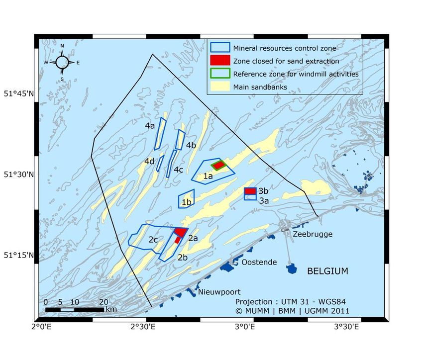
CONTENTS

1.       INTRODUCTION                                                               4

2.       CHARACTERISTICS OF THE BELGIAN PART OF THE NORTH SEA
                                                            6
         2.1 Physical and chemical characteristics          6
                 2.1.1     Seabed relief and bathymetry                             6
                 2.1.2     Hydrodynamics                                            7
                 2.1.3     Wind and wave action                                     8
                 2.1.4     Temperature                                             10
                 2.1.5     Turbidity                                               11
                 2.1.6     Salinity                                                12
                 2.1.7     Water masses and residence time                         13
                 2.1.8     Nutrients and oxygen                                    14
                 2.1.9     pH, pCO2 and sea acidification                          16
         2.2     Types of habitat                                                  19
                 2.2.1     Seabed                                                  19
                 2.2.2     Water column                                            19
                 2.2.3     Special habitats (Habitat Directive)                    20
                 2.2.4     Habitats requiring a specific protective regime         24
         2.3     Biological characteristics                                        25
                 2.3.1     Seabed                                                  26
                 2.3.2     Water column (phytoplankton, zooplankton, gelatinous
                           plankton)                                               31
                 2.3.3     Angiosperms, macroalgae                                 34
                 2.3.4     Fish populations                                        34
                 2.3.5     Sea mammals                                             37
                 2.3.6     Seabirds and Birds Directive                            38
                 2.3.7     Non-indigenous species introduced through human
                           activities                                              40
                 2.3.8     Other species listed under Community legislation or
                           international conventions                               41
         2.4     Alarming chemical pollution                                       43
                 2.4.1. Scope and evaluation                                       43
                 2.4.2. Current status quo                                         43

3.       PRESSURES AND IMPACTS                                                     46
         3.1  Physical destruction                                                 46
                 3.1.1     Port infrastructures and dredging works                 46
                 3.1.2     Wind farms                                              46
         3.2     Physical damage                                                   47
                 3.2.1     Fishery activities                                      47
                 3.2.2     Aggregate extraction                                    47
                 3.2.3     Maintenance dredging works and dumping of dredged
                           materials                                               50

     2   Initial Assessment for the Belgian marine waters - Directive 2008/56/EC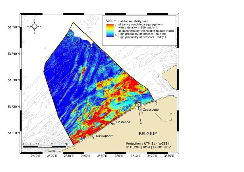
3.2.4     Morphological changes
                           (Bay of Heist, erosion Zeebrugge)                         52
         3.3     Physical disturbance                                                54
                 3.3.1     Underwater noise                                          54
                 3.3.2     Marine litter                                             54
                 3.3.3     Climate change                                            55
         3.4     Pollution from hazardous substances                                 55
                 3.4.1     Introduction of synthetics and heavy metals               56
                 3.4.2     Pollution caused by ships (carbon dioxide)                58
                 3.4.3     Introduction of radionuclides                             59
                 3.4.4     Chemical effects from the dumping of dredged material     61
         3.5     Enrichment with nutrients and organic substances                    61
         3.6     Biological disturbance                                              63
                 3.6.1     Introduction of microbial pathogens                       63
                 3.6.2     Non-indigenous species introduced by human activities     63
                 3.6.3     Selective extraction of species and bycatch               64
                 3.6.4     Wind farms                                                65
                 3.6.5     Biological disturbance as a result of sand extraction     66
                 3.6.6     Biological effects from the dumping of dredged material   67

4.       CONCLUSIONS                                                                 68

5.       REFERENCES                                                                  69

6.       MAP WITH PLACE NAMES                                                        79

7.       COLOPHON                                                                    80

     3   Initial Assessment for the Belgian marine waters - Directive 2008/56/EC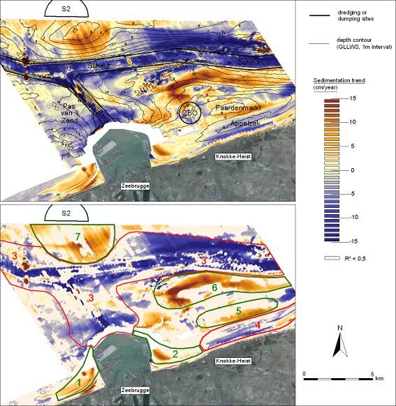
1. INTRODUCTION
The European Marine Strategy Framework Directive (2008/56/EC) lays down common
principles based on which the Member States must implement their own policies to achieve
good environmental status in the sea by 2020. Its aim is to protect and, if necessary, restore
the marine ecosystems in all of Europe.
The Member States must begin by describing the initial status of their waters: what is the
current status and which human activities affect that status? Next, the "good environmental
status" of the marine areas must be determined. This describes the situation we want
to/have to evolve towards in the near future. Finally, the Member States must define
measures to achieve the good environmental status.
This document provides an analysis of the initial status in the Belgian waters, describing the
physical, chemical and biological characteristics of our marine areas, as well as the human
activities that affect those areas. The report gives a limited reflection of the current status
and does not hold an assessment about the 'good environmental status' as described in the
report mentioned in articles 9 and 10. The 2010 Quality Status Report published by OSPAR
(OSPAR, 2010) forms the reference for the report.
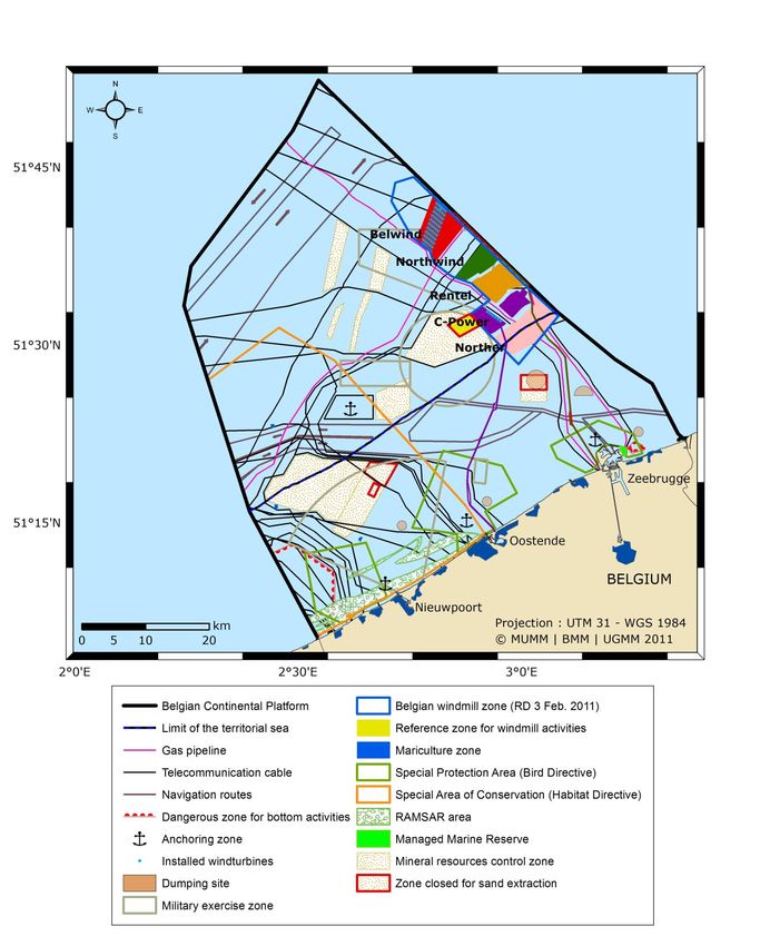
The Belgian Continental Shelf (BCS) has two distinct features: it is open and "very busy". As
for the openness: the status of the BCS depends more on the transboundary currents than on
the processes taking place within the zone itself. This means that Belgian responsibility for
the quality of its marine ecosystems is not without limits, which again illustrates the
importance of European and international collaboration. Although the area is small (3 454
km²), it hosts a large variety of activities: busy international sea routes; port activities; wind
farms; fishery; sand and gravel reclamation; mariculture; dredging and dumping of dredged
materials; military activities; recreational boating, etc.
4 Initial Assessment for the Belgian marine waters - Directive 2008/56/EC
Figure 1: the Belgian Continental Shelf.

     5   Initial Assessment for the Belgian marine waters - Directive 2008/56/EC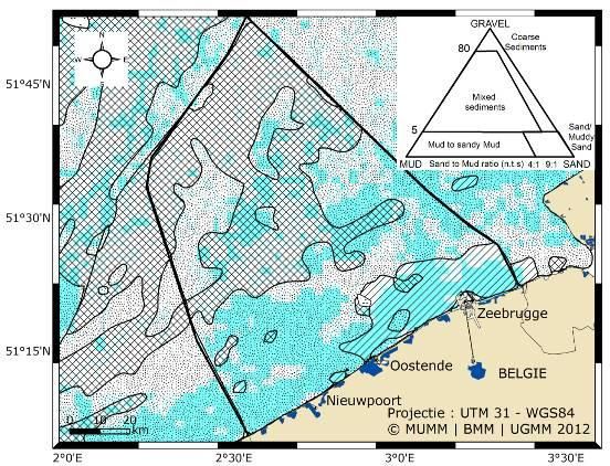
2. CHARACTERISTICS OF THE BELGIAN PART OF THE NORTH SEA
2.1. Physical and chemical characteristics
2.1.1 Seabed relief and bathymetry

Figure 2.1 shows the bathymetry of the seabed across the 3 454 km 2 of Belgian coastal
waters. In the near coastal area the water depth is usually less than 20 m, increasing to
approximately 45 metres further off the coast. Characteristic of the seabed is the existence of
sandbanks that run in a parallel to upward slanting pattern relative to the coast. Stretching 15
to 30 km, they can reach heights of approximately 20 metres from the bottom of the sea.

The substrate of the BCS consists mainly of sand and added clay, silt and gravel. Silt deposits
occur in the coastal area between Ostend and the Dutch border and originate from the
Holocene period, while Tertiary clay layers outcrop in a few deeper channels (Le Bot et al.
2005; Fettweis et al. 2009). The sandbanks coarsen from fine to coarse sand in a seaward
direction (Verfaillie et al. 2006).

Figure 2.1: Bathymetry of the BCS.

Putting together sedimentological, bathymetric and hydrodynamic data also allows for
distinguishing a few marine landscapes, often with ecological relevance (Verfaillie et al.
2009), see figure 2.2. Landscape 1 (yellow) is shallow and consists mainly of clay and silt.
Landscape 2 (light green) is shallow and consists of fine sand. Landscape 3 (dark green)
differs from zone 2 largely in that its sand is a gradient coarser. These landscapes mainly
match the slopes of the shallow, south-west facing sandbanks. The landscapes 4 (light

     6   Initial Assessment for the Belgian marine waters - Directive 2008/56/EC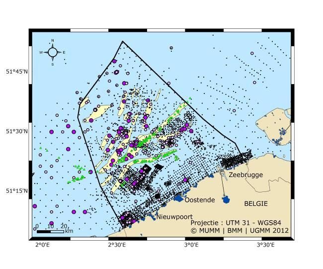
brown) and 5 (dark brown) consist of medium-coarse sand and they coincide with deep
terraces and the foot of the slopes of distant sandbanks (on the north-western and south-
eastern slopes, respectively). Landscapes 6 (light blue) and 7 (dark blue) coincide with the
ridges and the upper part of the slopes of deep sandbanks. Finally, landscape 8 (light grey)
consists mostly of gravel and pieces of shell. Fine-scale geomorphological mapping of sandy
substrates shows that slopes often coincide with higher biodiversity (Van Lancker et al.
2012).

Figure 2.2: Categorisation of the seabed into eight marine landscapes (Verfaillie et al. 2009).

2.1.2. Hydrodynamics

The hydrodynamics of the BCS is dominated by the daily tides, which can vary from as much
as 3 metres during neap tide to over 4.5 metres at spring tide. The tidal streams are intense,
often more than 1 m/s and in the coastal area they mainly occur parallel to the coast. The
presence of sandbanks changes the orientation in places, creating tide channels that differ at
ebb and flow. In addition, human activities such as the Zeebrugge port expansion and the
deepening of the sea lanes towards the ports of Ostend, Zeebrugge and the Scheldt estuary
have also affected the streams locally. These changes in hydrodynamics have in turn caused
or enhanced other phenomena, including the silting up of the Paardenmarkt east of
Zeebrugge (Van den Eynde et al. 2010).

Apart from the tides, wind and storms exert considerable impact on hydrodynamics. For
instance: a depression can change water transport, salinity, warmth or nutrients; it can cause
water level rises of several metres (2.25 m in Ostend before the 1953 Storm, Dehenauw
2003), bring about considerable increases in wave height and turbulence within the water
column and suspend large amounts of sediment.

Finally, the combination of the shallowness of the BCS and strong currents ensures
continuous mixing of the water column. If we exclude the extraordinary dynamics of the

     7   Initial Assessment for the Belgian marine waters - Directive 2008/56/EC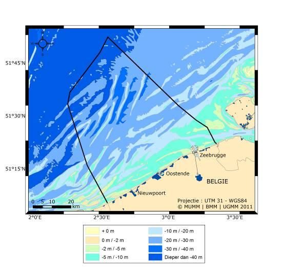
estuaries and of the Rhine and Meuse plume from the equation, the density gradients of sea
water are too small to cause important baroclinic currents.

Figure 2.3: General diagram of the circulation in the Channel and the southern part of the
North Sea. The black arrows represent the annual average residual circulation. The red
arrows show the horizontal dispersion, caused by the tide, on the transport of the Scheldt
and Rhine/Meuse water masses.

2.1.3. Wind and wave action

Besides the tides, meteorological conditions such as wind, precipitation, clouds, air
temperature near the marine surface, etc., are the most important causes of the physical
processes along our coastline. They usually follow a seasonal cycle, including a significant
variability of a few hours to several days that is associated with the passage of depressions.
The latter can have a significant impact on hydrodynamics. The inter-annual variability of the
meteorological parameters is correlated to the NAO index (North Atlantic Oscillation). This
variability also explains the differences in many oceanographic parameters such as the
temperature or transport of water masses in Belgian waters (Breton et al. 2006). However,
the flow rate of rivers such as the Scheldt is not correlated to the NAO index (Levy et al.
2010).

Figure 2.4 reflects the climatology of the winds, measured between 2000 and 2009 at the
Zeebrugge meteorological station. The average wind speed is 5.5 m/s. Weaker winds

     8   Initial Assessment for the Belgian marine waters - Directive 2008/56/EC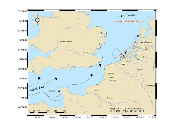
(
15 m/s, 5% of the time) mainly come from the west and south-west. The waves are closely
connected to the wind. The Belgian waters are considered to be moderately exposed to the
waves.

Figure 2.4: Wind rose for Zeebrugge from 2000 to 2009. The black line indicates the
orientation in relation to the coast (Baeye et al. 2011).

Figure 2.5 shows the significant wave height between 1999 and 2009, adjusted from Delgado
et al. (2010) and Matthys et al. (2011). Wave distribution at the offshore station Westhinder
is bimodal with a dominant direction caused by winds from the south-west and a second
direction caused by the winds blowing parallel to the North Sea axis (from north-north-east to
south-south-west). Wave distribution at the coastal station Bol van Heist is unimodal and
oriented towards the south-east.

Figure 2.5: Cumulative distribution of the significant wave height at Westhinder (left) and Bol
van Heist (right) in the period 1999-2009 (Fernandez et al. 2010).

     9   Initial Assessment for the Belgian marine waters - Directive 2008/56/EC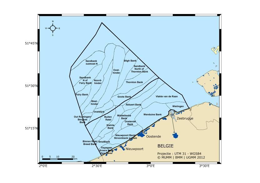
2.1.4. Temperature

The temperature of the sea water at the BCS shows a seasonal cycle with a clear difference
of approximately 15 °C between winter and summer temperatures (figure 2.6).

Figure 2.6: Average surface temperature in the period between 2005 and 2010 at the stations
Westhinder (above) and Bol van Heist (below). Source: "Meetnet Vlaamse Banken"
(Monitoring Network Flemish Banks) (Agency for Maritime Services, Coast Division).

The seawater temperature has an inter-annual variability of 1 to 4 °C and is strongly
correlated to the NAO index (Tsimplis et al. 2006).

    10   Initial Assessment for the Belgian marine waters - Directive 2008/56/EC
Figure 2.7 shows the spatial variation of the monthly averages of the surface temperature at the end of the winter (February) and in the summer (August). In winter, the warmer water masses originating from the Channel cause a temperature difference of 1 to 3 °C between the centre part of the southern bay of the North Sea and the coastal area. A turnaround can be perceived in the summer – with warmer water in the coastal area – as a result of the quick rise in temperature of the water in the more shallow coastal waters (Ruddick and Lacroix 2006). Figure 2.7: Monthly average surface temperature in the period 1995 to 2010. Left: February; right: August. Source: Bundesamt für Seeschiffahrt & Hydrographie (Loewe 2003). In general, the water at the BCS is well-mixed vertically with vertical temperature variations usually smaller than 0.5 °C. 2.1.5. Turbidity The BCS is characterised by a turbidity maximum along the entire coast. Turbidity is an optical parameter (the opposite of transparency) and is determined mainly by the concentration of suspended particulate matter SPM in our coastal waters. Here, concentrations of these mineral and organic substances are always high: from 100 mg/l up to several thousands of mg/l. There is also a transition area where SPM concentrations can be high (5-50 mg/l) and an offshore area where SPM concentrations are always low (
Figure 2.8: Turbidity map of the BCS - averages over the period 2003 until 2010. Turbidity
was calculated from the water reflectance that was measured by the MERIS satellite in the
665 nm band, using the tele-detection algorithm of Nechad et al. (2010) on MarCoast data.
The SPM concentration is in proportion with the turbidity.

2.1.6. Salinity

Figure 2.9 shows the long-term average salinity distribution in the southern part of the North
Sea and in the Channel. At this scale the difference between precipitation and evaporation is
negligible and therefore salinity in the coastal zone is affected mainly by the inflow of fresh
water from the big rivers.
The river plumes of the Scheldt, the Seine, the Rhine and the Meuse, with widths of up to 40
km, and of a few smaller rivers are visible along the coast. Here, salinity may vary between
25 and 32. For comparison: seawater entering the Channel has a salinity of approximately 35.

Changes in salinity in the long term are subject to the wind that may either push the river
plumes far into the sea, or stop them along the coast. The seasonal wind cycle, precipitation
and the flow rate of the rivers also cause seasonal changes in salinity along the Belgian coast.
Because the coastal area is well mixed vertically, vertical variations in salinity are usually
limited too (< 0.2).

    12   Initial Assessment for the Belgian marine waters - Directive 2008/56/EC
Figure 2.9: Salinity in the long term in the southern part of the North Sea and the Channel.
Left: average salinity measured on board the Belgica in the period 2005-2010. Right:
modelled average salinity in the period 1993-2010 (recalculated according to Lacroix et al.
2004). The figures in the circles represent the average in situ measured values.
2.1.7. Water masses and persistence
In the coastal zone, it is useful to define the concept of 'water mass' in relation to its origin.
This enables defining the origin of several polluting passive substances, dissolved in
seawater.
The transport of water masses is controlled mainly by residual tidal currents on the one hand
and currents caused by the wind on the other. In a weak wind, the residual transport in the
Belgian coastal zone typically flows from France to the Netherlands. However, the half-daily
oscillation of the tidal currents significantly increases the horizontal spread of the water
masses (Lacroix et al. 2004). This spread is more significant in the direction parallel to the
coast and may be the cause of transport of a water mass, salt and other nutrients in the
direction opposite to the residual currents (see figure 2.3).
Models show that water from the Atlantic Ocean is the main ingredient – 95% – in seawater
samples taken far from the coast. The remaining elements originate from freshwater from the
Scheldt, Rhine/Meuse, Seine and other small rivers (Lacroix et al. 2004).
The relative importance of the contribution of the Seine increases significantly in samples
taken further away from the coast. Also, for the larger part of the Belgian coastal zone, the
influence of the Rhine and the Meuse water masses at least equals that of the Scheldt water
masses.
Residence time θr is the average time needed by a water mass within a domain, to leave that
domain for the first time. Exposure period θ e is the average time a water mass remains within
an area. Exposure time exceeds residence time if – once away from the area – the water
mass returns into the area. The return coefficient can be defined as (θ r - θe)/θe (de Brye et al.
2011). The coefficient is 0 if not one single water part returns to the area, and 1 if all water
masses return to the calculated area.
13 Initial Assessment for the Belgian marine waters - Directive 2008/56/ECAs shown in figures 2.10 and 2.11, the residence time for the BCS is somewhere between 0
and 7 days. Exposure time is between 1 and 11 days and the return coefficient lies between
0.2 and 0.9. These figures show that the BCS is an open area with great influences from the
neighbouring areas.
Figure 2.10: Residence time (left) and exposure time (right) for the BCS.
Figure 2.11: Return coefficient for the BCS.
2.1.8. Nutrients and oxygen
Nutrients and oxygen are two of the main elements supporting the marine ecosystem. To be
able to perform photosynthesis and hence to grow, phytoplankton needs light and nutrients
(Nitrogen N, Phosphorus P, and for the diatoms dissolved Silicon Si). Although the biomass of
water plants constitutes no more than 1% of the biomass of all plants on earth, 40% of the
annual photosynthesis takes place in an aqueous environment. Despite considerable aquatic
productivity, this storage difference has to do with the fact that unicellular marine algae grow
14 Initial Assessment for the Belgian marine waters - Directive 2008/56/ECand die within a short time span (week-season-year), whereas the biomass of onshore plants
can be stored year after year. Similar to the systems on the shore, part of the organic
material created during the photosynthesis is transferred to higher levels in the food chain
(zooplankton, zoobenthos, fish, marine mammals, birds). When phytoplankton dies, the
organic material that is not transferred to the food chain is broken down by bacteria.
Dissolved oxygen is consumed during this recycling process and the organic material is again
transformed into inorganic nutrients (N and P).
Nutrients and oxygen are very important at the BCS in view of the problem of eutrophication,
a phenomenon directly resulting from an excess of nutrients and which can lead to a
shortage or even total absence of oxygen. Nutrient and oxygen levels have been monitored
for many years in the scope of the analysis of and fight against eutrophication throughout the
entire OSPAR region.
Despite the fact that nutrient levels exceed the limits, they do not cause shortage of oxygen
in the coastal waters, not even during the spring growth. This is illustrated in figure 2.12,
showing the evolution of oxygen saturation in the period 1995-2010. The diagram clearly
demonstrates that the situation is good (oxygen saturation continues to be over 70%) and
stable.
140
Zuurstofverzadiging in W05
130
Zuurstofverzadiging (%)
120
110
100
90
80
70
01-1995 01-1998 01-2001 01-2004 01-2007 01-2010
Figure 2.12: Oxygen saturation of the Belgian coastal waters in the period 1995-2010.
Throughout the Belgian coastal waters, concentrations of Dissolved Inorganic Nitrogen DIN
and Dissolved Inorganic Phosphorus DIP were compared to their regional background
concentrations. The DIN and DIP winter values exceed the limits of 15 µmol/l and 0.8 µmol/l
in large parts of the coastal waters. DIN and DIP concentrations as well as silicium
concentrations are highest near the Scheldt estuary and decrease in a south-west direction.
15 Initial Assessment for the Belgian marine waters - Directive 2008/56/EC150 120
DIN in W04 DIN in W05
120
90
Concentratie (µmol/l)
Concentratie (µmol/l)
90
60
60
30
30
0 0
01-1987 01-1991 01-1995 01-1999 01-2003 01-2007 01-2011 01-1987 01-1991 01-1995 01-1999 01-2003 01-2007 01-2011
5 5
DIP in W05
DIP in W04
4 4
Concentratie (µmol/l)
Concentratie (µmol/l)
3 3
2 2
1 1
0 0
01-1990 01-1994 01-1998 01-2002 01-2006 01-2010 01-1990 01-1994 01-1998 01-2002 01-2006 01-2010
Figure 2.13: DIN and DIP concentrations between 1988 and 2010 at station W04 (Zeebrugge,
Scheldt influence) and W05 (further from the coast).
A statistically significant trend in DIN concentrations was not observed between 1974 and
2010. There was, however, a shift in the balance between nitrate/nitrite and ammonium and
a slight decrease in silicium concentrations. The most remarkable trend is the significant fall
in DIP concentrations, which can be explained from a decrease of P load. This evolution
resulted in important shifts in the relationships that determine the growth of phytoplankton
and diatoms. The decrease in DIP concentrations resulted in a strong DIN overweight as
compared to DIP and Si. In fact, this means that the phosphate concentration currently
constitutes the limiting factor for phytoplankton growth and that the silicium concentration is
the limiting factor for diatoms.
2.1.9. pH, pCO2 and acidification of the sea
Carbon chemistry was researched using in situ measurements (Borges and Frankignoulle
1999; 2002; 2003; Schiettecatte et al. 2006; Borges et al. 2008) and modelling (Gypens et al.
2004; 2009; 2011; Borges and Gypens 2010). Carbon chemistry is strongly influenced by the
freshwater plume of the Scheldt estuary, with salinity lying between approximately 29 and
35. This causes strong spatial gradients in carbon chemistry, as is shown in figure 2.14,
where data of the Scheldt estuary is compared to data collected further at sea. The water
column is well-mixed throughout the year, which eliminates the occurrence of vertical
gradients in carbon variables.
The seasonal variations in carbon chemistry parameters are caused by the intake and release
of CO2, as shown in the positive correlation between partial CO 2-pressure (pCO2) and
16 Initial Assessment for the Belgian marine waters - Directive 2008/56/ECdissolved inorganic carbon (DIC), and the negative correlation between pCO 2 and pH, and
pCO2 and calcite saturation. The key factors in this context are: the supply of water from the
Scheldt estuary with low pH and high CO2, leading to low pH and high pCO2-levels in the
winter; phytoplankton growth in the spring, leading to low pCO 2 and high pH-levels; the
decomposition of organic materials later in the summer and the fall, leading to maximum
pCO2 and minimum pH-levels in the fall. The supply of highly alkaline water from the Scheldt
not only controls CO2, but also the DIC-levels (Frankignoulle et al. 1996; Borges et al. 2008).
800 8.5
700
SSS ~ 29
8.4
600
pCO2 (ppm)
500 8.3
pH
400 8.2
300 SSS ~ 35
8.1
200
100 8.0
J F M A M J J A S O N D J F M A M J J A S O N D
2600 7
6
DIC (µmol kg -1)
2400
calcite
5
2200
4
2000
3
1800 2
J F M A M J J A S O N D J F M A M J J A S O N D
Figure 2.14: Climatological seasonal variations of partial CO 2-pressure (pCO2), pH, dissolved
inorganic carbon (DIC) and calcite saturation (Ωcalcite) at the Scheldt estuary (surface salinity
approximately 29) and the furthest offshore part of the BCS (surface salinity approximately
35) (Borges and Frankignoulle 1999; 2002; Borges et al. 2008).
The existing time series do not allow for studies of long-term (10-100 years) changes in
carbon chemistry. Biogeochemical models, however, permit the creation of historical
reconstructions. Changes in the carbon cycle in the period 1951 to 1998 as a result of an
increase in atmospheric CO2 and of the nutrient supply by rivers were studied using the R-
MIRO-CO2 model (Gypens et al. 2009; Borges and Gypens 2010). Three periods can be
distinguished between 1951 and 1988 based on the N and P loads in rivers, the quality of
nutrient enrichment (defined as the relation DIN:PO 4 during the winter), the gross primary
production (GPP), the net community production (NCP) and the air-sea CO2-fluxes.
From 1951 to 1965, the annual increase in both the nutrient supply from rivers and the GPP
was small, and NCP and air-sea CO2-fluxes remained stable. From 1965 to 1990, nutrient
supply increased and the winter relation DIN:PO4 roughly met the phytoplankton needs
(Redfield relation = 16:1), causing the GPP and NCP to increase and BCS to change from a
source of CO2 to a pit for atmospheric CO 2. From 1990 to 1998, the decreased P load of the
rivers – mainly due to the removal of polyphosphates from washing detergents – led to
winter relations DIN:PO4 exceeding the Redfield relation, causing P to become a limiting
factor and resulting in a decrease in primary production. The BCS changed from a net
autotrophic system into a net heterotrophic system and from a pit into a source of
atmospheric CO2.
Between 1965 and 1990, when nutrient supply from rivers grew and the winter relation
DIN:PO4 roughly coincided with the Redfield relation, pH and Ωcalcite increased as a result of
17 Initial Assessment for the Belgian marine waters - Directive 2008/56/ECthe rise in GPP. After 1990, GPP fell, as did pH and Ωcalcite. As a result, eutrophication and the
corresponding changes in the carbon cycle (rise of GPP and a shift from net heterotrophy to
net autotrophy) affected the marine carbon chemistry, which in turn neutralised the carbon
chemistry of the acidification of oceans.
After 1990, when GPP again fell, the decrease in pH and Ω calcite was significantly greater than
could be expected from the simple increase in atmospheric CO 2. The post-1990 trends can be
explained from the ecosystem's quick change from net autotrophic to net heterotrophic, in
relation with the – limiting, in terms of primary production – rise of the rise of the DIN:PO4.
This shift to net heterotrophy led to a net annual CO 2-production at the ecosystem level, with
a strong effect on the marine carbon chemistry. This emphasises the fact that changes in
river nutrient load as a result of management measures can alter the carbon cycle in the
coastal zone considerably, even to an extent that temporarily, greater changes would arise in
the carbon chemistry than the ones caused by the acidification of the ocean.
Based on existing data (see above as well as non-published data from Borges), the current
situation shows the same patterns as those in the late 1990s: net heterotrophy; net CO 2
emissions into the atmosphere; changes in carbon chemistry occur quicker than might be
expected from the increase of atmospheric CO 2 only. In other words: the net biomass
consumption exceeds net biomass production, resulting in the sea emitting CO2.
35 5 1.5
air-sea CO 2 flux (mmol m -2 d-1)
total N inputs
30
Total N inputs (kTN yr -1)
Total P inputs (kTP yr -1)
total P inputs 1.0
4
25
0.5
20 3
0.0
15 2
-0.5
10
1 -1.0
5
0 0 -1.5
40 8.20
30
8.15
DIN:PO4
pH
20
Redfield ratio 8.10
10 Atmopsheric CO 2
increase alone
0 8.05
120 4 3.5
100
NCP (mmol C m -2 d-1)
GPP (mmol C m -2 d-1)
GPP 2
80
calcite
60 0 3.0
40
NCP
-2
20
Atmopsheric CO 2
0 -4 increase alone
2.5
1955 1965 1975 1985 1995 1955 1965 1975 1985 1995
Figure 2.15: Evolution between 1951 and 1998 of the annual total N and P loads from the
Scheldt, winter DIN:PO4, calculated using the R-MIRO-CO2 model; total primary production
(GPP), net community production (NCP), air-sea CO2-fluxes, pH and calcite saturation (Ωcalcite)
(according to Gypens et al 2009; Borges and Gypens 2010).
18 Initial Assessment for the Belgian marine waters - Directive 2008/56/EC2.2. Types of habitat
Characteristic for the BCS is its complex system of sandbanks that, based on their orientation
and depth, can be categorised into four different types. The closest system, the Kustbanken
[Coast banks], lie parallel to the coastline and stretch from the beach several kilometres into
the sea. At low tide, the peaks of these sandbanks are only a few metres deep. Some of them
even fall dry at low tide. The Vlaamse Banken consist of a series of parallel, south-west to
north-east oriented banks. They are located some 10 to 30 metres from the coast. At low
tide, the tops of these banks are at a depth of four metres on average. Parallel to the
coastline and at a distance of 15 to 30 kilometres are the Zeelandbanken or Zeeuwse Banken
(Zeeland banks). With very few exceptions, the tops of these banks lie below the 10 m
isobath. And lastly, there is the Hinderbanken system, some 35 to 60 kilometres from the
coast. These sandbanks have a south-west to north-east orientation and just like the Zeeland
Banks, are located below the 10 m isobath.
2.2.1 Seabed
The mobile substrates of the Belgian Part of the North Sea BPNS consist of a gradient of
sediment types, varying from cohesive silt via fine sand towards coarser permeable
sediments. This strong gradient in sediment composition is responsible for the relatively high
diversity of benthic biotopes. There are four subtidal benthic biotopes, each named after their
characteristic macrobenthic organisms: the Macoma balthica biotope; the Abra alba biotope;
the Nephtys cirrosa biotope and the Ophelia borealis biotope. Each of these biotopes is
inhabited by a specific macrobenthic, epibenthic and fish fauna.
Besides these mobile substrates, non-mobile beds such as tertiary clay and turf beds and
gravel beds outcrop in several places. These types of habitat are also characterised by a
specific fauna, based on which several biotopes were distinguished. The Barnea candida
biotope is known from tertiary clay banks in the coastal area, but can also occur in offshore
turf banks. Whereas the aforementioned biotopes are typically inhabited by burrowed fauna
and free-living surface dwellers, the gravel beds form the biotope of attached and associated
organisms.
Many areas also contain artificial structures, such as breakwaters, shipwrecks, port walls and
the more recent wind turbine parks. In terms of structure, the fauna of these biotopes is
closely associated to that of the natural hard substrates, i.e. the gravel beds. Differences as
compared to the gravel beds are related to the type of substrate, their geographic location
and their exposure to currents.
19 Initial Assessment for the Belgian marine waters - Directive 2008/56/ECFigure 2.16: Predicted spread of the four subtidal macrobenthic biotopes: light grey: low
chance of occurrence; dark grey: high chance of occurrence; white: not predicted. A:
Macoma balthica biotope; B: Abra alba biotope; C: Nephtys cirrosa biotope; D: Ophelia
borealis biotope (Degraer et al. 2008). Projection UTM 31N – WGS84.
2.2.2. Water column
The water column, also known as the pelagia, is the largest maritime biotope in Belgium. At
the top of the pelagia is the photic zone, where vegetable phytoplankton performs its
photosynthesis. This phytoplankton forms the basis of the pelagic food chain and is predated
by zooplankton, which in turn plays a crucial role for higher trophic levels (fish). The
zooplankton consists of small animal organisms free-floating in the water column. We
distinguish holoplankton (that live in the water column their entire life) and meroplankton
(that only spend part of their life cycle in the water column). Many benthic organisms have
meroplanktonic larvae, creating a clear connection between the pelagic and benthic
ecosystems. At the BCS we find several plankton communities closer to the coast, as well as
in deeper waters where the water column contains less detritus and the inflow of Atlantic
water ensures a greater presence of oceanic zooplankton species (e.g. krill). The
holoplankton is dominated mainly by calanoid copepods ( Temora longicornis, Acartia clausi,
Centropages hamatus, Paracalanus parvus, Calanus helgolandicus ). Jellyfish constitute a
second large holoplanktonic group, such as the greatly expanding comb jelly Mnemiopsis
leidyi. Significant meroplanktonic groups are the larvae of crabs, shrimp, fish and
echinoderms.
20 Initial Assessment for the Belgian marine waters - Directive 2008/56/ECMigrating pelagic fish species such as herring, sprat, mackerel and horse mackerel feed on
zooplankton. Juvenile herring and sprat inhabit our coast banks throughout the year. Adult
herring can be found here later in the year, when the fish are passing on their way to their
spawning grounds in the Channel (large schools of fish). Two other key pelagic species show
up during summer and autumn: the mackerel and horse mackerel. Horse mackerel breeds on
the BCS, with juveniles abundant in the offshore pelagic fish community.
Due to its function as a breeding ground and high turnover, the pelagia plays a key role in
the operation of our marine food chain, but it is highly affected by changes in seawater
temperature, oceanic inflow and nutrient concentrations.
2.2.3 Special habitats (Habitat Directive)
Two types of habitats as laid down in Annex 1 of the Habitat Directive occur at the BCS:
sandbanks slightly covered by seawater all the time (habitat type 1110) and reefs (habitat
type 1170).
Habitat type 1110 is described as the structurally and functionally indivisible aggregate of
sandbank top and flanking channels such as they can be distinguished morphologically on
bathymetric maps. Since from a morphological point of view, practically the entire BCS can be
considered as a system of sandbanks and channels, this habitat type stretches a distance of
3148 km². Only in the northern part do the sandbanks gradually roll into a sand wave field,
which is the reason why this area is not classified as Habitat type 1110. We distinguish 24
different sandbank systems.
Two habitat types 1170 associated with habitat type 1110 occur as well: the geogenic gravel
beds and the biogenic Lanice conchilega aggregates. Gravel beds are generally recognised as
areas of special ecological value: they are home to a rich flora and fauna and contain a high
biodiversity of stones. For instance, the European oyster Ostrea edulis, a reef forming
species from the southern North Sea that is now threatened with extinction, appears to be
highly dependent on gravel beds. Gravel beds also have a key function as breeding and
growing area for various fish species.
Aggregates of the sand mason worm L. conchilega cause local sediment accumulations,
creating clearly marked structures with specific physical characteristics. Within these
aggregates, the macrobenthic biodiversity is four to six times higher than the surrounding
sediment, while the macrobenthic density exceeds it by 34 times. Furthermore, the
aggregates are an important foraging and shelter area for, among others, juvenile flat fish.
21 Initial Assessment for the Belgian marine waters - Directive 2008/56/ECFigure 2.17: Spatial distribution of habitat type 1110 indicating the 24 sandbank
systems (Degraer et al. 2009).
22 Initial Assessment for the Belgian marine waters - Directive 2008/56/ECFigure 2.18: Mapping of potential gravel areas (yellow zones), sample areas (purple),
observed gravel areas (green) (Degraer et al. 2009).
23 Initial Assessment for the Belgian marine waters - Directive 2008/56/ECFigure 2.19: Habitat suitability map for Lanice conchilega aggregates with a density of >
500 ind/m² as generated using the MaxEnt programme for habitat suitability modelling. Most
likely absent: blue (0); most likely present: red (1) (Degraer et al. 2009).
2.2.4 Habitats requiring a specific protective regime
Based on the occurrence and spread of the habitat type from Annex 1 of the Habitat
Directive: "sandbanks slightly covered by seawater all the time" (habitat type 1110), two
marine protected areas were already indicated in 2004: the Trapegeer-Stroombank area and
Vlakte van de Raan. In February 2008, the Belgian Council of State rescinded the
establishment of the Vlakte van de Raan. In 2010, the Trapegeer-Stroombank area was
expanded at the request of the European Union: the indicated Vlaamse Banken area
comprises both habitat type 1110 and the associated habitat type 1170.
Table 2.1: Absolute surface of Habitat types 1110 "sandbanks slightly covered by seawater all
the time", including characteristic benthic biotopes, and 1170 "reefs" as described in the
Habitat Directive area "Vlaamse Banken" (Flemish Banks).
Habitat type / Biotope Surface area
Habitat type 1110 1,107 km²
Macoma balthica biotope 24 km²
Abra alba biotope 245 km²
Nephtys cirrosa biotope 521 km²
Ophelia borealis biotope 292 km²
Habitat type 1170, associated with habitat type 1110
Gravel beds 221 km²
Lanice conchilega aggregates ± 285 km²
The selected sandbanks within the suggested Habitat Directive area all fall in the range of
sandbanks with the highest ecological value in terms of one or more of the four benthic
24 Initial Assessment for the Belgian marine waters - Directive 2008/56/ECbiotopes. The area also comprises a considerable part of the surface of habitat type 1170.
Besides its benthic importance, the area of the Habitat Directive is also known as a breeding
ground for, among others, fish species of commercial importance.
Figure 2.20: Geographical location of the protected areas.
2.3. Biological characteristics
Marine biodiversity can be defined as the variety of living marine organisms and the
ecological complexes they form part of. It is hard to estimate the species richness of marine
organisms at the BCS. Some one hundred thousand species have been identified in the North
Sea basin, but estimates put the number of species inhabiting the area at no less than three
million. 2,187 marine species were counted at the BCS (Vandepitte 2010). Zooming in on the
macrobenthos (i.e. macroscopic organisms living in and on the seabed), the BCP is definitely
not one of the richest systems in the North Sea basin (Rees et al., 2007) and it has a
regionally typical low species richness. Still, in 2005 the number of observed macrobenthic
species was estimated at 265 for the mobile substrates and 224 for the non-mobile substrates
(Degraer et al. 2006, Zintzen and Massin 2010).
25 Initial Assessment for the Belgian marine waters - Directive 2008/56/EC2.3.1. Seabed The Belgian part of the North Sea consists of three large substrate types that in ecological terms coincide with a EUNIS level 3 habitat classification (figure 2.21). EUNIS is a hierarchic system for classifying habitats in Europe and its surrounding seas. There are six levels with marine habitats discriminated mainly according to biological zone (littoral, infralittoral, circalittoral, etc.), substrate type, hydrodynamic energy (wave exposure, tidal force), oceanographic variables (salinity) and the typical biological species. EUNIS A5.1 habitats are coarse-grained sediments; A5.2 is the sand to muddy sand category; A5.3 is mud to sandy mud; and A5.4 is the mixed sediment category (Van Lancker 2012). The coarse-grained substrates comprise the gravel beds, except for the large blocks that have been included in the gravel mapping (figure 2.18). The reliability of the demarcation of these substrate types decreases in a seaward direction. The occurrence of EUNIS level 3 marine habitats is available for the north-eastern part of the Atlantic Ocean (Cameron and Askew 2011). Figure 2.21: The occurrence of EUNIS level 3 habitats at the BPNS. The mapping is based on the relations between the percentages of gravel, sand and mud (see caption) (nts: not to scale): coarse-grained sediments (shaded area) consist of either >=80% gravel, or of sediments with a sand/mud ratio ≥ 9; sand to muddy sand (dots) is made of
Soft substrates

The macrobenthic communities in the mobile or soft substrates form a key indicator of the
health of the marine ecosystem. Four subtidal communities are distinguished, each associated
with a specific habitat: the Macoma balthica community; the Abra alba community; the
Nephtys cirrosa community and the Ophelia borealis community (Degraer et al. 2003; 2008;
Van Hoey et al. 2004). These communities do not occur as isolated entities: there are gradual
transitions between them.

  Macoma balthica                   Abra alba                  Nephtys cirrosa     Ophelia borealis

Figure 2.22: Habitus of the characteristic and descriptive types of the four macrobenthic
communities living in the non-mobile or soft substrates of the BCS.

A very low density (190 ind/m² on average) and species richness (5 spp/0.1 m² on average)
are typical for the O. borealis bristle worm community that can be found in medium- to
coarse-grained seabeds. Another characteristic species is the interstitial bristle worm
Hesionura elongata.

The N. cirrosa bristle worm community has a low density (402 ind/m² on average) and a low
species richness (7 spp/0.1 m² on average) and typically lives in fine to medium sandy
sediments that are very low in silt. Other characteristic species include the bulldozer
amphipod Urothoe poseidonis and the sand digger shrimp Bathyporeia spp.

The M. balthica (tellin) community features low species richness (on average 7 spp/0.1 m²)
but relatively high density (on average 967 ind/m²); its typical finding place is in silty
sediments. The M. balthica community is closely related to the A. alba community: three of
the most common species are also found in the A. alba community. Characteristic species
include: the bristle worms Cirratulidae and Heteromastus filiformis. A likely explanation for
the lower species richness in the eastern coastal waters is the high concentration of
suspended matter.

Finally, the A. alba community is characterised by a large density (6,432 ind/m² on average),
a high species richness (30 spp/0.1 m² on average) and it is typically found in fine sand rich
in silt. Characteristic species include the white furrow shell Abra alba, the cut through shell
Spisula subtruncata, the bivalve mollusc Mysella (Kurtiella) bidentata, the caprellid Pariambus
typicus, as well as bristle worms, including Stenelais boa and the “reef” building sand mason
worm Lanice conchilega. The A. alba community also harbours an abundance of the invasive
American jackknife Ensis directus (Houziaux et al. 2012). First found in 1987, this species now
displays average densities of 9 ind/m² in coastal waters (Houziaux pers. comm.).

                                     Figure 2.23: After a storm, the shells of the white furrow
                                     shell Abra alba frequently wash ashore. The photo also
                                     shows specimen of the American jackknife Ensis directus, as
                                     well as a Baltic tellin Macoma balthica.

    27   Initial Assessment for the Belgian marine waters - Directive 2008/56/EC
The benthic communities show significant annual variation as a result of seasonal fluctuation,
varying degrees of success in recruitment, cold winters and changing sediment composition
(Van Hoey et al. 2007). Due to, among other things, a lack of continuity in long-term
monitoring, the scope and causes of these variations largely remain unknown.
Within the A. alba community, for instance, a shift in community structure was observed
between the periods 1995-1997 and 1999-2003, probably caused by changes in the
hydroclimatic North Sea environment (Van Hoey et al. 2007). In the first (unstable) period,
the community structure was defined by, e.g., a varying degree of success of recruitment,
cold winters and changing sediment composition, while the second (stable) period was
characterised rather by regular seasonal fluctuations in community composition. Other
examples of long/longer-term variation include the fluctuations in numbers and densities of
general species such as the cut through shell Spisula subtruncata, the common cockle
Cerastoderma edule, the banded wedge-shell Donax vittatus, the various species of flat shells
Tellina spp., the trumpet worm Pectinaria koreni and the sand mason worm L. conchilega.
During the last two decades, the benthic communities in the coastal waters underwent
significant changes as a result of the introduction of non-indigenous species. At the same
time, several other species such as the otter shell Lutraria lutraria and the common netted
dog whelk Nassarius reticulatus became much more abundant. And finally, several southern
species expanded their terrain into the Belgian coastal waters and became increasingly
numerous. Despite the fact that many of these species wash onto our shores in great
numbers, most of the changes go unnoticed in the current benthos study, probably because
the applied technology does not or inadequately sample certain - e.g. deep sea - species.
For the longer term, a comparison of the actual situation to the fauna of bivalved species
collected by G. Gilson at the beginning of the 20th century (KBIN collection) shows that the
situation has changed (Van Lancker et al, 2012). In general we see a regression of the pure
sand species (Donax vittatus, Mactra stultorum, Spisula solida ) and a clear expansion of the
species that prefer more silty environments (e.g. A. alba, M. balthica, Fabulina fabula, and
other species). These observations suggest siltation of the coastal sediments, probably as a
result of an increase in maritime and port activities. In addition the average richness of
bivalved species seems to have increased. This phenomenon is probably related to the
organic enrichment which has been characteristic for the southern part of the North Sea since
the second half of the 20th century.
These soft substrates make a significant contribution to the functioning of the ecosystem
(Vanaverbeke et al. 2011; Braeckman 2011). This mainly has to do with activities of
bioturbation and bio-irrigation that also determine the nature of the macrobenthic
communities. Bioturbation and bio-irrigation (i.e. functional diversity) are crucial transport
mechanisms for the carbon and nitrogen cycles in fine-sanded sediments that are subject to a
high influx of organic material. A fall in bioturbators leads to decreased processing of organic
materials in the seabed, while a decline in bio-irrigators results in reduced oxygen exchange
and denitrification, which largely helps towards compensating nitrogen eutrophication in
shallow seas. These characteristics are important for the integrity of the seabed.
Especially the Abra alba community contains a number of important bioturbators and bio-
irrigators that play a considerable role in the global nutrient cycle and thus can increase the
densities and diversities of the infauna (Braeckman, 2011). In this context, L. conchilega is a
significant bio-irrigator with the strongest impact on oxygen exchange in the sediment. The
exchange stimulates mineralisation processes: the release of nutrients and denitrification are
doubled as compared to seabeds that have no fauna. High densities of A. alba are important
for the bioturbation potential, or burying organic material, while L. conchilega colonies will
lead to continued denitrification. Consequently, both bioturbation and bio-irrigation are key
elements in the functioning of the benthic ecosystem (Braeckman, 2011). Because cohesive
silt has a more limited pore-water exchange than fine sands, only certain communities can
survive (e.g. M. balthica).
28 Initial Assessment for the Belgian marine waters - Directive 2008/56/ECNatural hard substrates
Several studies have found that gravel beds harbour a rich flora and fauna with a high
species richness of both infauna and epifauna on the grit (e.g. Kühne and Rachor 1969;
Davoult and Richard 1988; de Kluijver 1991; Dahl and Dahl 2002; Van Moorsel 2003). Those
rich communities can only develop if the habitat is not strongly subject to natural and/or
andropogenic disturbance.
Studies at the BCS mainly involved the gravel beds near the Hinderbanken and the Vlaamse
Banken (Houziaux et al. 2008, Van Lancker et al. 2007). Gravel is found mainly in between
the channels between the banks. The gravel beds near the Hinderbanken have special
importance: historical data from the Gibson collection indicates that at the end of the 19 th
century, gravel beds were the most dominant type of habitat in the channel between the
Oosthinder and Westhinder and that they harboured a very high biodiversity (Van Beneden
1883, Houziaux et al. 2008). This data further shows a clear correlation between the spread
of the gravel beds and that of the European oyster Ostrea edulis (Houziaux et al. 2008), a
species currently practically extinct in the southern North Sea. It is assumed that these oyster
beds acted as source population for the intertidal oyster populations (Houziaux et al. 2008).
Together with the grit, the oysters were colonised by a highly diverse epifauna (e.g.
Pomatoceros triqueter, Sabellaria spinulosa, Haliclona occulata, Flustra foliacea, Alcyonidium
spp., Alcyonium digitatum, Sertularia cupressina, Nemertesia spp.), and numerous other
smaller and more mobile species lived there as well. As such they constituted the ultimate hot
spot of benthic biodiversity at the BCS (Houziaux et al. 2008).
Comparisons with the current species composition of the macrobenthos indicate that
considerable changes have taken place in species compositions (Houziaux et al. 2008), e.g.
(1) a probable change from moss animals (Bryozoa, one of them being Flustra, Alcyonidium
spp.) to a Hydrozoa-dominated system (such as Organ pipe hydroid Tubularia spp.) and (2) a
change from dominance of long-living species (such as the oyster Ostrea edulis and the whelk
Buccinum undatum) towards shorter-living, opportunistic species (e.g. starfish Asterias
rubens, serpent star Ophiura spp. and brittle star Ophiothrix fragilis). The nature of the
observed changes shows that they are at least partly related to the constant disturbance of
the seabed due to fishery activities. And yet, various typical species are still being found, e.g.
painted top shell Calliostoma zizyphinum and dead man's fingers A. digitatum. Particularly the
fauna of species that drill through stones and live in cavities, such as Barnea parva,
Gastrochaena dubia, Kellia suborbicularis en Hiatella spp.), is unique.
29 Initial Assessment for the Belgian marine waters - Directive 2008/56/ECFigure 2.24: Example of a fauna associated with gravel beds.
Recently in two small zones near the Hinderbanken a remarkably well-developed fauna of
gravel beds was found, with a well-developed layer of three-dimensional epifauna species,
such as sponges, moss animals and hydropolyps, which in turn harbour a more mobile fauna
of, among others, sea sludges, small crustaceans and worms (Houziaux et al. 2008). It is
highly likely that their location gives these places a natural shield against seabed disturbing
human activities (beam trawling). This refuge offers an insight into the possible ecological
potential of the Belgian gravel banks if the pressure from operations on the seabed were to
be reduced.
Finally, another characteristic of the BCS is the sporadic occurrence of turf banks and
outcropping banks of tertiary clay. These natural and non-mobile substrates harbour a
separate, yet species-poor macrobenthic community, its typical species including drilling
bivalves such as the white piddock Barnea candida and the (non-indigenous) American
piddock Petricola pholadiformis (Degraer et al. 1999). This community shows a migration in
several parts, both in time and in area, due to its direct dependence on the presence of the
above-mentioned non-mobile substrates.
Artificial hard substrates
Coastal artificial hard substrates such as breakwaters, dikes and other coastal defence works
constitute the habitat for a community similar to that living in natural rock formations,
characterised by a high species richness and biomass (Engledow et al. 2001). It is the only
place where large benthic brown seaweeds Phaeophyta, larger red seaweeds Rhodophyta
and green seaweeds Chlorophyta are found. The prevalent community there is typical for a
medium-exposed rocky coast, characterised by barnacles (e.g. Semibalanus balanoides,
Balanus crenatus and Elminius modestus), a dense mussel zone (Mytilus edulis) and, to a
lesser extent, a zone consisting of brown seaweeds. Numerous other invertebrates live
among the mussels. This community can be considered as a depleted reflection of the one
existing on the French and English Channel coasts as large brown seaweeds such as
Laminaria spp. and Himanthalia elongata, as well as the characteristic low red seaweed zone
are absent from the Belgian coast.
231 obstructions were identified on the BCS, most of them shipwrecks (Zintzen et al. 2006;
Mallefet et al. 2008). These artificial hard substrates are often colonised by a community that
is different from the ones found in the surrounding areas. In terms of biomass, the fauna on
shipwrecks largely consists of Cnidaria (coelenterates), whereas Amphipoda dominate in
terms of density (Zintzen et al. 2008). Three communities were distinguished: in the coastal
area the Metridium senile (sea anemone) community with a limited number of species,
together with the somewhat richer community of Tubularia larynx (organ pipe hydroid);
further from the coast, the fouling community is dominated by Tubularia indivisa (oaten pipes
30 Initial Assessment for the Belgian marine waters - Directive 2008/56/EChydroid). Tubularia spp. (a mixture of Tubularia indivisa and Tubularia larynx) on the wrecks
are always associated with the tube-building amphipod Jassa herdmani. A total of about one
hundred species were found on and around the shipwrecks, many of them belonging to rare
taxa (Zintzen et al. 2006).
Figure 2.25: Three-dimensional vegetation
on the artificial hard substrates associated
with the offshore wind farms at the BCS.
Installation of wind parks on the BCS started in 2008. Contrary to the artificial hard substrates
in the coastal zone, these substrates are found mainly in clear waters and the hard substrate
stretches from the sandy seabed (to a depth of 30 m) and above the supralittoral fringe. This
produces a clear zoning pattern, characterised by a higher diversity of biotopes and species
(Kerckhof et al. 2009, 2010). The deeper parts of the subtidal are dominantly inhabited by
the moss animal Electra pilosa, amidst smaller mobile species such as the crab Pisidia
longicornis, the bristle worm Autolytus sp. and amphipoda Jassa spp. and Aora gracilis. This
community forms the diet of large numbers of fish, such as the pout Trisopterus luscus (up to
30,000 individuals per wind turbine) and cod Gadus morhua that are drawn to these parks
(Reubens et al. 2010, 2011). The shallow subtidal and the low intertidal zones mainly harbour
the amphipod Jassa spp. and the barnacle Balanus perforatus, whereas the species-poor
higher intertidal zone houses little more than the marine splash midge Telmatogeton
japonicus (besides a few macro algae species).
2.3.2. Water column (phytoplankton, zooplankton, gelatinous plankton)
The annual plankton growth cycle starts early spring with a growth of diatoms (Rousseau et
al. 2002). In April and May, the algal bloom mainly comprises the colony-forming slime algae
Phaeocystis globosa (Lancelot et al. 1987) (Haptophyta) which is capable of producing a large
quantity of biomass (foam). In June, both the diatoms and Phaeocystis disappear from the
water column (Rousseau et al. 2002), most probably as a result of nutrient shortage and
possibly also of an enhanced predation pressure of heterotrophic plankton species such as
the dinoflagellate Noctiluca scintillans (Daro et al. 2006). A second, less extensive diatom
bloom occurs later in the summer and in the autumn (Rousseau et al. 2002).
31 Initial Assessment for the Belgian marine waters - Directive 2008/56/ECFigure 2.26: Seasonal distribution of the phyto- and zooplankton in the central zone of the
BCS: average results over the period 1988-2004, (a) Phytoplankton: colonies of Phaeocystis
(red) and diatoms (green). (b) Zooplankton: microprotozooplankton (grey), copepods (bruin)
and sea sparkle N. scintillans (blue) (Daro et al. 2006).
The spatial variability of the spring peak in chlorophyll a concentrations, which is an indicator
of phytoplankton biomass, reflects the spatial variability of nutrients during the winter
(Muylaert et al. 2006; Brion et al. 2006; Rousseau et al. 2006). The annual variability in
amplitude and period of the diatoms and Phaeocystis bloom is affected by meteorological
factors (wind, river flow rate) as characterised by the NAO index (Breton et al. 2006).
Based on research that was carried out in the scope of the OSPAR strategy "Eutrophication",
the Water Framework Directive (WFD European Union 2000) defines the quantity of
phytoplankton as one of the elements of biological water quality in relation to eutrophication.
For application of the WFD to the coastal waters (European Union 2008), threshold values for
chlorophyll a of 10 µg/l and 15 µg/l were used to distinguish between a "very good to good"
and "good to average" environmental status. These threshold values apply to the 90th
percentile of the chlorophyll a measurements during the bloom season.
Figure 2.27 shows the indicator as derived from satellite data. The colour red represents an
average environmental situation, whereas orange stands for "good" and green for "very
good". Blue reflects the oceanographic conditions.
32 Initial Assessment for the Belgian marine waters - Directive 2008/56/ECYou can also read