INTEGRAZIONE GEOMETRICA NUMERICA PER PROBLEMI STOCASTICI DI EVOLUZIONE - INDAM
←
→
Page content transcription
If your browser does not render page correctly, please read the page content below
Integrazione geometrica numerica
per problemi stocastici di evoluzione

           Raffaele D’Ambrosio
        DISIM - Università dell’Aquila

            Congresso GNCS
          Montecatini, 11–13 febbraio 2020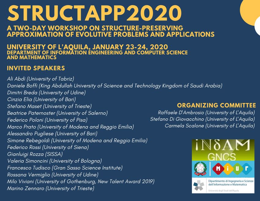
Progetto GNCS 2018: Progetto GNCS 2019:
“Approssimazione numerica di “Problemi di evoluzione e loro
problemi di evoluzione: aspetti discretizzazione: questioni di
deterministici e stocastici”; stabilità lineare e non lineare”.
Aspetti numerici nei problemi evolutivi (e.g., problemi
stocastici, sistemi discontinui, ODEs matriciali, equazioni
con ritardo, PDEs che generano fronti d’onda periodici, ...);
vari inserti di algebra lineare numerica, ottimizzazione
numerica, teoria dei sistemi dinamici;
numerose applicazioni (e.g., oscillatori chimici accoppiati,
dinamica delle popolazioni, matrix completion nei sistemi di
raccomandazione, biomatematica, teoria dei grafi, ...).
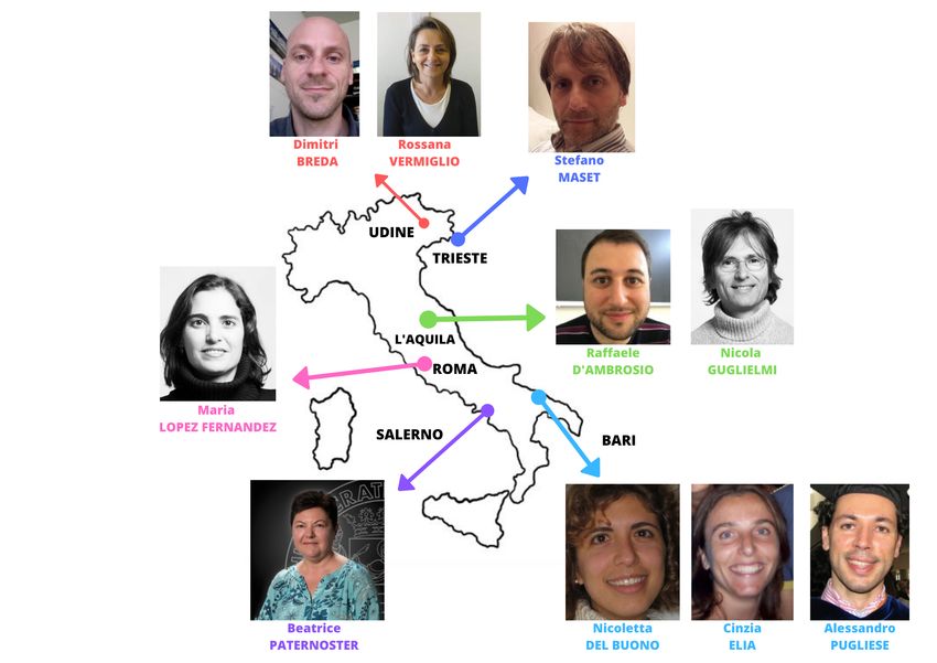
Partecipanti non strutturati:
Alessia Andò (Udine, 2018 e 2019), Asma Farooq (Trieste 2019), Da-
vide Liessi (Udine, 2018), Martina Moccaldi (Salerno, 2018), Francesca
Scarabel (Helsinki, 2018 e 2019), Simone Spada (Trieste, 2018 e 2019).

Pubblicazioni nel biennio 2018–2019
 Andreotti, E., Edelmann, D., Guglielmi, N., Lubich, C. Constrained graph partitioning via
 matrix differential equations, SIAM Journal on Matrix Analysis and Applications 40(1),
 1–22 (2019).

 Banjai, L., López-Fernández, M. Efficient high order algorithms for fractional integrals and
 fractional differential equations, Numerische Mathematik 141(2), 289–317 (2019).

 Boccarelli, A., Esposito, F., Coluccia, M., Frassanito M.A., Vacca, A., Del Buono, N.
 Improving knowledge on the activation of bone marrow fibroblasts in MGUS and MM
 disease through the automatic extraction of genes via a nonnegative matrix factorization
 approach on gene expression profiles, Journal of Translational Medicine 16(1),217 (2018).

 Bohinc, K., Reščič, J., Spada, S., May, S., Maset, S. Influence of added salt on the surface
 induced ordering of nanoparticles with discretely distributed charges, Journal of Molecular
 Liquids 294,111134 (2019).

 Breda, D., Liessi, D. Approximation of eigenvalues of evolution operators for linear renewal
 equations, SIAM Journal on Numerical Analysis 56(3), 1456–1481 (2018).

 Breda, D., Menegon, G., Nonino, M. Delay equations and characteristic roots: Stability and
 more from a single curve, Electronic Journal of Qualitative Theory of Differential Equations,
 89 (2018).

 Cesarone, F., Pepe, P., Guglielmi, N. Solution by sampled-data control of a consensus
 problem: An approach by stabilization in the sample-and-hold sense, Proceedings of the
 American Control Conference 8430969, 6493–6498 (2018).
Pubblicazioni nel biennio 2018–2019
 Cardone, A., Conte, D., D’Ambrosio, R., Paternoster, B. Stability issues for selected
 stochastic evolutionary problems: A review, Axioms 7(4),91 (2018).

 Cardone, A., Conte, D., D’Ambrosio, R., Paternoster, B. Collocation methods for volterra
 integral and integro-differential equations: A review, Axioms 7(3),45 (2018).

 Cardone, A., Conte, D., D’Ambrosio, R., Paternoster, B. On quadrature formulas for
 oscillatory evolutionary problems, International Journal of Circuits, Systems and Signal
 Processing 12, 58–64 (2018).

 Cardone, A., Conte, D., Paternoster, B. Two-step collocation methods for fractional
 differential equations, Discrete and Continuous Dynamical Systems - Series B 23(7),
 2709–2725 (2018).

 Cardone, A., D’Ambrosio, R., Paternoster, B. A spectral method for stochastic fractional
 differential equations, Applied Numerical Mathematics 139, 115–119 (2019).

 Casalino, G., Castiello, C., Del Buono, N., Mencar, C. A framework for intelligent Twitter
 data analysis with non-negative matrix factorization, International Journal of Web
 Information Systems 14(3), 334–356 (2018).

 Cicone, A., Guglielmi, N., Protasov, V.Y. Linear switched dynamical systems on graphs,
 Nonlinear Analysis: Hybrid Systems 29, 165–186 (2018).

 Citro, V., D’Ambrosio, R. Long-term analysis of stochastic θ-methods for damped stochastic
 oscillators, Applied Numerical Mathematics (2019).
Pubblicazioni nel biennio 2018–2019
 Colombo, A., Del Buono, N., Lopez, L., Pugliese, A. Computational techniques to locate
 crossing/sliding regions and their sets of attraction in non-smooth dynamical systems,
 Discrete and Continuous Dynamical Systems - Series B 23(7), 2911–2934 (2018).

 Conte, D., D’Ambrosio, R., Moccaldi, M., Paternoster, B. Adapted explicit two-step peer
 methods, Journal of Numerical Mathematics 27(2), 69–83 (2019).

 Conte, D., D’Ambrosio, R., Paternoster, B. On the stability of ϑ-methods for stochastic
 volterra integral equations, Discrete and Continuous Dynamical Systems - Series B 23(7),
 2695–2708 (2018).

 Conte, D., Paternoster, B., Moradi, L., Mohammadi, F. Construction of exponentially fitted
 explicit peer methods, International Journal of Circuits, Systems and Signal Processing 13,
 501–506 (2019).

 D’Ambrosio, R., Moccaldi, M., Paternoster, B., Rossi, F. Adapted numerical modelling of
 the Belousov–Zhabotinsky reaction, Journal of Mathematical Chemistry 56(10), 2876–2897
 (2018).

 D’Ambrosio, R., Moccaldi, M., Paternoster, B., Rossi, F. Stochastic numerical models of
 oscillatory phenomena, Communications in Computer and Information Science 830, 59–69
 (2018).

 D’Ambrosio, R., Moccaldi, M., Paternoster, B. Numerical preservation of long-term
 dynamics by stochastic two-step methods, Discrete and Continuous Dynamical Systems -
 Series B 23(7), 2763–2773 (2018).
Pubblicazioni nel biennio 2018–2019
 D’Ambrosio, R., Moccaldi, M., Paternoster, B. Parameter estimation in
 IMEX-trigonometrically fitted methods for the numerical solution of reaction–diffusion
 problems, Computer Physics Communications 226, 55–66 (2018).

 D’Ambrosio, R., Paternoster, B. Multivalue collocation methods free from order reduction,
 Journal of Computational and Applied Mathematics, in press (2019).

 Del Buono, N., Elia, C., Garrappa, R., Pugliese, A. Preface: “structural dynamical systems:
 Computational aspects”, Discrete and Continuous Dynamical Systems - Series B 23(7), i
 (2018).

 Dieci, L., Eirola, T., Elia, C. Periodic orbits of planar discontinuous system under
 discretization, Discrete and Continuous Dynamical Systems - Series B 23(7), 2743–2762
 (2018).

 Dieci, L., Elia, C. Smooth to discontinuous systems: A geometric and numerical method for
 slow-fast dynamics, Discrete and Continuous Dynamical Systems - Series B 23(7), 2935–2950
 (2018).

 Dieci, L., Papini, A., Pugliese, A. Coalescing points for eigenvalues of banded matrices
 depending on parameters with application to banded random matrix functions, Numerical
 Algorithms 80(4), 1241–1266 (2019).

 Elia, C., Maroto, I., Núñez, C., Obaya, R. Existence of global attractor for a
 nonautonomous state-dependent delay differential equation of neuronal type,
 Communications in Nonlinear Science and Numerical Simulation 78,104874 (2019).
Pubblicazioni nel biennio 2018–2019
 Esposito, F., Gillis, N., Del Buono, N. Orthogonal joint sparse NMF for microarray data
 analysis, Journal of Mathematical Biology 79(1), 223–247 (2019).

 Fazzi, A., Guglielmi, N., Markovsky, I. An ODE-based method for computing the
 approximate greatest common divisor of polynomials, Numerical Algorithms 81(2), 719–740
 (2019).

 Guglielmi, N., Manetta, M. Stability of gyroscopic systems with respect to perturbations,
 Springer INdAM Series 30, 253–266 (2019).

 Guglielmi, N., Mason, O., Wirth, F. Barabanov norms, Lipschitz continuity and
 monotonicity for the max algebraic joint spectral radius, Linear Algebra and Its
 Applications 550, 37–58 (2018).

 Guglielmi, N., Protasov, V.Y. On the closest stable/unstable nonnegative matrix and related
 stability radii, SIAM Journal on Matrix Analysis and Applications 39(4), 1642–1669 (2018).

 Guglielmi, N., Scalone, C. Computing the closest real normal matrix and normal
 completion, Advances in Computational Mathematics, in press (2019).

 Gyllenberg, M., Scarabel, F., Vermiglio, R. Equations with infinite delay: Numerical
 bifurcation analysis via pseudospectral discretization, Applied Mathematics and
 Computation 333, 490–505 (2018).

 Lopez, L., Maset, S. Time-transformations for the event location in discontinuous ODEs,
 Mathematics of Computation 87(313), 2321–2341 (2018).
Pubblicazioni nel biennio 2018–2019
 Markovsky, I., Fazzi, A., Guglielmi, N. Applications of polynomial common factor
 computation in signal processing, Lecture Notes in Computer Science (including subseries
 Lecture Notes in Artificial Intelligence and Lecture Notes in Bioinformatics) 10891, 99–106
 (2018).

 Maset, S. Conditioning and relative error propagation in linear autonomous ordinary
 differential equations, Discrete and Continuous Dynamical Systems - Series B 23(7),
 2879–2909 (2018).

 Sadeghpour, M., Breda, D., Orosz, G. Stability of Linear Continuous-Time Systems with
 Stochastically Switching Delays, IEEE Transactions on Automatic Control 64(11), 8665935,
 4741–4747 (2019).

 Scalone, C., Guglielmi, N. A gradient system for low rank matrix completion, Axioms 7(3),
 51 (2018).

 Spada, S., Maset, S., Bohinc, K. Interaction between like-charged surfaces mediated by
 uniformly charged counter-nanoparticles, International Journal of Modern Physics B
 33(10),1950092 (2019).

 Citro, V., D’Ambrosio, R., Di Giovacchino, S. A-stability preserving perturbation of
 Runge-Kutta methods for stochastic differential equations, Appl. Math. Lett. (2019).

 Citro, V., D’Ambrosio, R. Nearly conservative multivalue methods with extended bounded
 parasitism, Appl. Numer. Math. (2019).
Discretizzazioni structure-preserving
                       Problemi deterministici
   Integrazione geometrico-numerica di problemi Hamiltoniani
   con E. Hairer (Ginevra); J. Butcher (Auckland);
   sistemi dinamici discontinui
   con L. Dieci (Georgia Tech), Fulbright; A. Scotti (Milano);
   PDEs che generano fronti d’onda periodici
   con B. Paternoster (Salerno).

                          Problemi stocastici
   Hamiltoniani
   con D. Cohen (Umea);
   non lineari (contrattività in media, oscillatori smorzati)
   con E. Buckwar (Linz); S. Di Giovacchino, C. Scalone (L’Aquila);
   con memoria
   con D. Conte e B. Paternoster (Salerno).
Integrazione geometrica (deterministica)
Problemi Hamiltoniani

      ẏ(t) = J ∇H(y(t)),          t ≥ 0,                 0 −I
                                                       J=        .
      y(0) = y0 ,                                         I 0
            "       #
                p(t)
   y(t) =               ∈ R2d , momenti e coordinate generalizzate;
                q(t)
   la funzione Hamiltoniana

                                     H : R2d → R

   è un integrale primo del problema, dunque

                             H(y(t)) = H(y0 ),     t ≥ 0.

   Infatti,
       d
          H(y(t)) = ∇H(y(t))T ẏ(t) = ∇H(y(t))T J −1 ∇H(y(t)) = 0.
       dt
Integratori simplettici
I metodi Runge-Kutta simplettici conservano esattamente
Hamiltoniane quadratiche;
se la soluzione numerica calcolata con un metodo Runge-Kutta di
ordine p giace in un insieme compatto, allora
H(yn ) = H(y0 ) + O(hp ),
per tempi lunghi (Benettin-Giorgilli, 1994);
metodi lineari multistep quasi-conservativi
a lungo termine (Hairer-Lubich, 2004);
metodi multivalue quasi conservativi a lungo termine (Butcher,
D’Ambrosio, 2017; D’Ambrosio, Hairer, 2013, 2014).Integratori simplettici
I metodi Runge-Kutta simplettici conservano esattamente
Hamiltoniane quadratiche;
se la soluzione numerica calcolata con un metodo Runge-Kutta di
ordine p giace in un insieme compatto, allora
H(yn ) = H(y0 ) + O(hp ),
per tempi lunghi (Benettin-Giorgilli, 1994);
metodi lineari multistep quasi-conservativi
a lungo termine (Hairer-Lubich, 2004);
metodi multivalue quasi conservativi a lungo termine (Butcher,
D’Ambrosio, 2017; D’Ambrosio, Hairer, 2013, 2014).
Esempio: pendolo semplice
p2
H(y) = − cos q.
2Pendolo semplice: spazio delle fasi
Runge-Kutta di Gauss a 2 stadi (simplettico)Pendolo semplice: spazio delle fasi (ctd.)
Eulero esplicito (non simplettico)Pendolo semplice: spazio delle fasi (ctd.)
Eulero esplicito (non simplettico)
Uri M. Ascher, Surprising computations, Appl. Numer. Math. (2012).Equazioni differenziali stocastiche
Problemi di Itō:
dX(t) = f (X(t))dt + g(X(t)) dW (t), t ≥ 0,
f : Rd → Rd (drift), g : Rd → Rd×m (diffusione),
W (t) processo di Wiener m-dimensionale.
Formulazione integrale:
Z t Z t
X(t) = X(0) + f (X(s))ds + g(X(s))dW (s) .
0 0
| {z }
integrale di Itō∗
*Su una rete uniforme {0 < t1 < t2 < · · · ≤ tn }, è definito come
n
X
lim g(X(tj ))(W (tj+1 ) − W (tj )).
n→∞
j=1
√
Incrementi di Wiener distribuiti come h · N (0, 1), con h = tj+1 − tj .Integrazione geometrica (stocastica)
Integrazione geometrica (stocastica)
   Invarianza di leggi asintotiche nella discretizzazione di sistemi
   lineari (Schurz, 1999);
   conservazione a lungo termine della densità stazionaria di
   oscillatori lineari smorzati, con rumore additivo (Burrage, Lythe,
   2007, 2009); D’Ambrosio, Moccaldi, Paternoster, 2018; Citro, D’Ambrosio, 2020);

   metodi partizionati per oscillatori lineari con rumore additivo
   (Melbo, Higham, 2004);

   oscillatore di Duffing stocastico       (Welfert, 2017);

   Runge-Kutta per Hamiltoniane stocastiche separabili                (Burrage
   2012, 2014).

   integrazione geometrica di problemi Hamiltoniani stocastici.

   C. Chen, D. Cohen, R. D’Ambrosio, A. Lang, Drift-preserving numerical
   integrators for stochastic Hamiltonian systems, Adv. Comp. Math.
   (2020).
Sistemi Hamiltoniani stocastici
Per Hamiltoniane della forma
                                1
                 H(p(t), q(t)) = pT p + V (q),   t ≥ 0,
                                2
con V : Rd → R potenziale sufficientemente regolare, consideriamo
                   dq(t) = p(t) dt
                   dp(t) = −V 0 (q(t)) dt + Σ dW (t).

con Σ ∈ Rd×m .
Sistemi Hamiltoniani stocastici
Per Hamiltoniane della forma
1
H(p(t), q(t)) = pT p + V (q), t ≥ 0,
2
con V : Rd → R potenziale sufficientemente regolare, consideriamo
dq(t) = p(t) dt
dp(t) = −V 0 (q(t)) dt + Σ dW (t).
con Σ ∈ Rd×m .
Legge invariante di traccia (Burrage, 2014)
1
E [H(p(t), q(t))] = E [H(p(t0 ), q(t0 ))] + Tr Σ> Σ t
2
Crescita lineare della funzione Hamiltonian attesa.Sistemi Hamiltoniani stocastici
Per Hamiltoniane della forma
1
H(p(t), q(t)) = pT p + V (q), t ≥ 0,
2
con V : Rd → R potenziale sufficientemente regolare, consideriamo
dq(t) = p(t) dt
dp(t) = −V 0 (q(t)) dt + Σ dW (t).
con Σ ∈ Rd×m .
Legge invariante di traccia (Burrage, 2014)
1
E [H(p(t), q(t))] = E [H(p(t0 ), q(t0 ))] + Tr Σ> Σ t
2
Crescita lineare della funzione Hamiltonian attesa.
Questa proprietà si conserva lungo discretizzazioni del sistema?Conservazione numerica della legge di traccia
In Burrage (2014) emerge (dalla sperimentazione) che
la perturbazione stocastica di metodi simplettici non conserva la
legge di traccia;
lo stesso accade per metodi energy-preserving.
V. Citro, R. D’Ambrosio, Long-term analysis of stochastic theta-methods
for damped stochastic oscillators, Appl. Numer Math. (2020).
Esempio: singolo processo di Wiener
dq(t) = p(t) dt
dp(t) = −V 0 (q(t)) dt + σ dW (t).
√
La parte lineare delle σ-espansioni di p e q contiene il σ t (termine
secolare).Conservazione numerica della legge di traccia
C. Chen, D. Cohen, R. D’Ambrosio, A. Lang, Drift-preserving numerical integrators for
stochastic Hamiltonian systems, Adv. Comp. Math. (2020).
Z 1
h
Ψn+1 = pn + Σ∆Wn − V 0 (qn + shΨn+1 )ds,
2 0
qn+1 = qn + hΨn+1 , (?)
Z 1
pn+1 = pn + Σ∆Wn − h V 0 (qn + shΨn+1 ) ds.
0
Teorema
Se V ∈ C 1 (Rd ), lo schema (?) soddisfa la legge di traccia
1
E [H(pn , qn )] = E [H(p(t0 ), q(t0 ))] + Tr Σ> Σ tn ,
2
per ogni tn = nh punto di rete.Conservazione numerica della legge di traccia
Teorema
Supponiamo V 0 Lipschitz continuo. Allora, esiste h∗ > 0 tale che, per
ogni 0 < h ≤ h∗ , lo schema numerico (?) converge con ordine 1 in
media quadratica,
1/2 1/2
E |q(tn ) − qn |2 + E |p(tn ) − pn |2
≤ Ch,
ove la costante C è indipendente da h e da n.
Altre proprietà
Analisi dell’errore in senso debole e forte;
analisi dell’errore in relazione allo stimatore del valore medio
(Monte Carlo, Monte Carlo multilevel, ...);
analisi dell’errore Hamiltoniano.Test numerici (pendolo stocastico)
1 √
H(p, q) = p2 − cos(q), σ = 0.25, (p0 , q0 ) = (1, 2).
2
0.6 0.7
EM DP
0.55 DP Exact
BEM
0.6
Exact
0.5
Energy Energy
0.45 0.5
0.4
0.4
0.35
0.3 0.3
0 1 2 3 4 5 0 5 10
Time TimeTest numerici (doppia buca di potenziale)
1 1 1 √ √
H(p, q) = p2 + q 4 − q 2 , ε = 0.5, (p0 , q0 ) = ( 2, 2).
2 4 2
8
DP
Exact
6
Energy
4
2
0
0 10 20 30 40 50
TimeTest numerici (Hénon-Heiles con doppio rumore)
1 2 2
1 2 2
2 1 3
H(p, q) = p + p2 + q + q2 + α q1 q2 − q1 ,
2 1 2 1 3
√
0.2 0 1 3
Σ= , p0 = , q0 = , α = 1/16.
0 0.2 1 1
5
DP
Exact
4.5
Energy
4
3.5
3
0 10 20 30 40 50
TimeConclusions Primi passi nell’integrazione geometrico-numerica di SDEs Conservazione di leggi invarianti Stabilità non lineare Altri operatori (SVIEs, SFDEs, oscillatori stocastici) E. Buckwar, R. D’Ambrosio, Exponential mean-square stability properties of stochastic linear multistep methods, submitted. C. Chen, D. Cohen, R. D’Ambrosio, A. Lang, Drift-preserving numerical integrators for stochastic Hamitlonian systems, Adv. Comput. Math. (2020). V. Citro, R. D’Ambrosio, Long-term analysis of stochastic theta-methods for damped stochastic oscillators, Appl. Numer Math. (2020). D. Conte, R. D’Ambrosio, B. Paternoster, On the stability of theta-methods for stochastic Volterra integral equations, Discr. Cont. Dyn. Sys.-B (2018). R. D’Ambrosio, S. Di Giovacchino, Mean-square contractivity of stochastic θ-methods, submitted. R. D’Ambrosio, M. Moccaldi, B. Paternoster, Numerical preservation of long-term dynamics by stochastic two-step methods, Discr. Cont. Dyn. Sys.-B (2018).
Assegni di ricerca a L’Aquila
PRIN2017-MIUR
“Structure preserving approximation of evolutionary problems”

Primo bando: giugno 2020

Tematiche: integrazione structure-preserving di problemi di evoluzione
deterministici e stocastici
Grazie per l’attenzione!
ε-espansioni
   Idea classica in ambito deterministico (e.g., problemi
   singolarmente perturbati; vedi Hairer, Wanner).
   Esempio (didattico):
                          x2 + 2εx − 1 = 0,       ε  1.
                 ∞
                 X
   Ansatz: x =         xn εn . Sostituendo nell’equazione e raccogliendo le
                 n=0
   potenze di ε, si ottiene
                          ε0 : x20 − 1 = 0
                          ε1 :    2x0 (x1 + 1) = 0
                          ε2 : x21 + 2x0 x2 + 2x1 = 0

                                                     ε2
                             x ≈ xε = ±1 − ε ±
                                                     2
                                       ε = 10−1   ε = 10−3
                       |x+   −   x+
                                  ε|    1.24e-5   1.25e-13
ε-espansioni
Consideriamo il problema test scalare
dq 0 −1 σ
= y dt + dW,
dp 1 0 0
corrispondente al problema del secondo ordine
q̈ = −q + σξ(t),
ove ξ(t) è un rumore Gaussiano. Generalmente, la letteratura considera
come problema test
√
q̈ = −q + ε t
con ε ∼ N (0, σ 2 ). Ansatz:
q(t) = q0 (t) + εq1 (t) + ε2 q2 (t) + . . .ε-expansions (ctd.)
Sostituendo nell’equazione e raccogliendo le potenze di ε, si ottiene
ε0 : q¨0 + q0 = 0
√
ε1 : q¨1 + q1 = t
..
.
Dunque,
! ! !
2√ 2√ √
r r r r
π π
q(t) = cos(t) + sin(t) − ε C t cos(t) + S t sin(t) + t + . . .
2 π 2 π
! ! !
2√ 2√
r r r
π
p(t) = cos(t) − sin(t) + ε C t sin(t) − S t cos(t) + . . .
2 π π
ove S e C sono le funzioni integrali di Fresnel
Z x π
S(x) = sin t2 dt,
2
Z0 x π
C(x) = cos t2 dt.
0 2ε-espansioni (ctd.)
! ! !
2√ 2√ √
r r r r
π π
q(t) = cos(t) + sin(t) − ε C t cos(t) + S t sin(t) + t + . . .
2 π 2 π
! ! !
2√ 2√
r r r
π
p(t) = cos(t) − sin(t) + ε C t sin(t) − S t cos(t) + . . .
2 π π
√
t: termine secolare;
nell’integrazione a lungo termine, la parte secolare è dominante;
nell’integrazione a lungo termine, la funziona Hamiltoniana
modificata (i.e., quella associata alla ε-espansione) differisce
significativamente da quella originale;
la conservazione di leggi invarianti, dunque, non è una
caratteristica generale dei metodi stocastici.Figure: Hamiltonian modificata attesa (rosso) VS Hamiltoniana attesa (blu) per ε = 0.01; 0.1; 0.2; 0.5.
You can also read