Introduction to Image Processing Cameras, lenses and sensors - Cosimo Distante
←
→
Page content transcription
If your browser does not render page correctly, please read the page content below
Computer
 Vision

              Introduction to Image
                    Processing

           Cameras, lenses and sensors

                    Cosimo Distante

                 Cosimo.distante@cnr.it
              Cosimo.distante@unisalento.it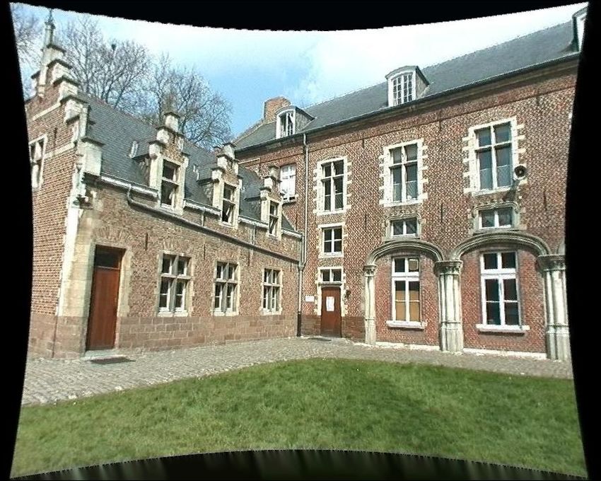
Computer
 Vision    Cameras, lenses and sensors

           • Camera Models
             – Pinhole Perspective Projection
           • Camera with Lenses
           • Sensing
           • The Human Eye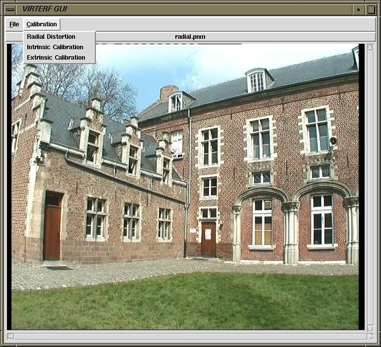
Computer Images are two-dimensional patterns of brightness values.
 Vision

               Figure from US Navy Manual of Basic Optics and Optical Instruments, prepared by Bureau of
               Naval Personnel. Reprinted by Dover Publications, Inc., 1969.

              They are formed by the projection of 3D objects.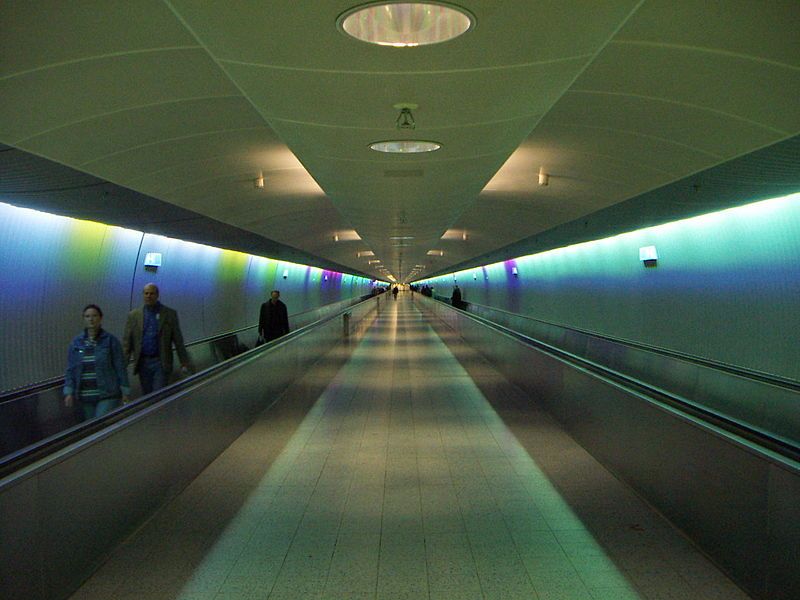
Computer
 Vision

           Animal eye:
                                           Photographic camera:
           a looonnng time ago.            Niepce, 1816.

                Pinhole perspective projection: Brunelleschi, XVth Century.
                Camera obscura: XVIth Century.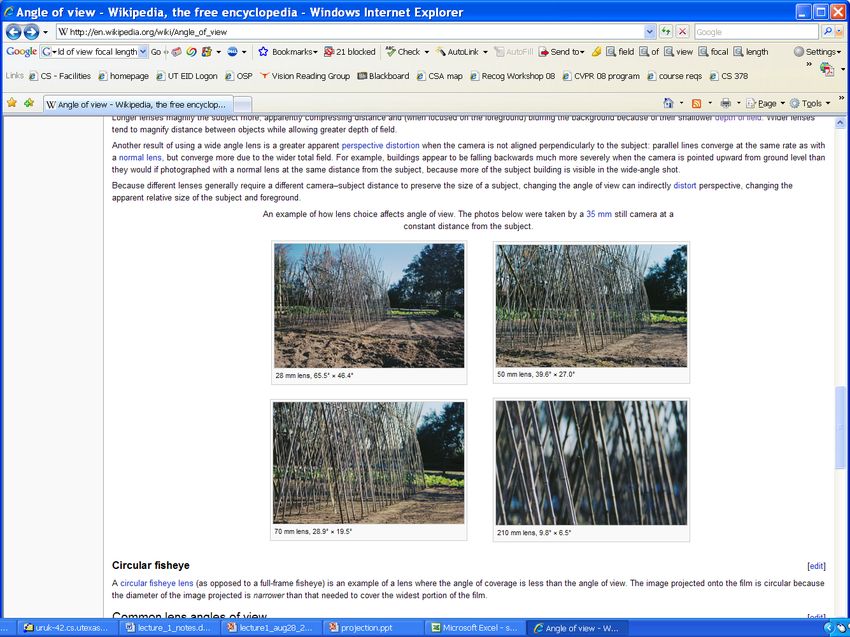
1.1.1    Perspective Projection
Computer
                              Pinhole model
           Imagine taking a box, using a pin to prick a small hole in the center of one of its
 Vision    sides, and then replacing the opposite side with a translucent plate. If you held
           that box in front of you in a dimly lit room, with the pinhole facing some light
           source, say a candle, you would observe an inverted image of the candle appearing
           on the translucent plate (Figure 1.2). This image is formed by light rays issued
           from the scene facing the box. If the pinhole were really reduced to a point (which
           is of course physically impossible), exactly one light ray would pass through each
           point in the image plane of the plate, the pinhole, and some scene point.

               image
               plane

                                             pinhole                      virtual
                                                                          image

                                  Figure 1.2. The pinhole imaging model.

               In reality, the pinhole will have a finite (albeit small) size, and each point in the
           image plane will collect light from a cone of rays sustending a finite solid angle, so
           this idealized and extremely simple model of the imaging geometry will not strictly
           apply. In addition, real cameras are normally equipped with lenses, which further
           complicates things. Still, the pinhole perspective (also called central perspective)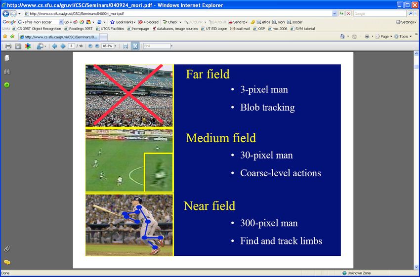
Computer
 Vision    Distant objects appear smaller

Computer
 Vision    Perspective effects
Computer
 Vision    Perspective effects

Computer
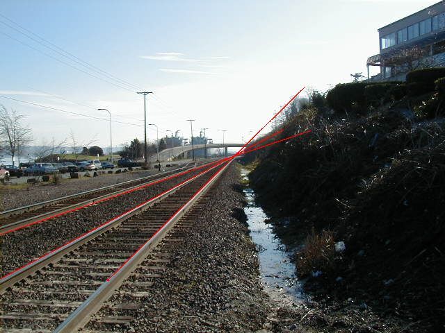
Vision Parallel lines meet
• vanishing point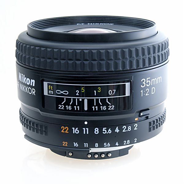
Computer
 Vision               Vanishing points

           Before beginning, we have to learn a
           couple of key concepts about linear
           perspective:
           •All lines vanishing at the same point are
           parallel.
           •We call horizontal lines those vanishing on
           the horizon, and vertical lines those that are
           perpendicular to the horizontal ones. It also
           can be defined the vertical lines as those that
           target the center of the earth, that is, as the
           line that forms the string of a plumb-line.
Computer
Vision Vanishing points
• In these images, the blue line represents the horizon and the
aquamarine circle in the center, the point of view of the observer.Computer
Vision Vanishing points
• Now we look a little upwards. We see that the verticals converge
into the sky, towards a vanishing point located above our head -
the zenithComputer
Vision Vanishing points
• And the opposite case. We look down and the verticals converge
on to the ground, towards a vanishing point located beneath our
feet - the nadir -Computer
Vision Vanishing points
• Now an example of frontal or parallel perspective. It is
characterized by having a single vanishing point, which lies on the
horizon and that will always match our view point.Computer
Vision Vanishing points
• Now we see an example with two vanishing points. These two
vanishing points are located on the horizon. As we also have our
view point on the horizon, the verticals do not converge.Computer
Vision Vanishing points
• And here we have an example with three vanishing points, and
now we look up above and see that the verticals have now
become convergentComputer
Vision Vanishing points
• And here we have an example with three vanishing points, and
now we look up above and see that the verticals have now
become convergent. The following image shows the opposite
case, when looking down.Computer
Vision Vanishing points
• And finally, look where the sides of the staircase converge. The
left wall converges on the horizon as it is horizontal, while the
sides of the staircase, being inclined, converge at a point located
above the horizon. In case they were inclined downwards, they
would converge towards a point located below the horizon.Computer
Vision Vanishing points
H VPL VPR
VP1 VP2
To different directions
correspond different vanishing points
VP3Computer
Vision Vanishing points
Application to autonomous navigation in critical conditions
Necessary to use other cues such as textureComputer
Vision Vanishing points
the focal length of the camera can be calculated from two
vanishing points associated with orthogonal scene directions
the orthocenter of the triangle formed by three vanishing
points associated with three orthogonal scene directions is
the principle point
Likewise, those same three vanishing points can be used to
determine both the internal camera parameters (under cer-
tain simplifying assumptions) and camera rotation
Even a single vanishing point can provide valuable
information about the camera modelComputer Vision Vanishing points
Computer
 Vision    Vanishing points
Computer
 Vision    Geometric properties of projection

           • Points go to points
           • Lines go to lines
           • Planes go to whole image
                             or half-plane
           • Polygons go to polygons

           • Degenerate cases:
              – line through focal point yields point
              – plane through focal point yields line
Computer
Vision Pinhole Camera Model
X p
Image plane
P=(X,Z)
P=(x,f) X
Optical axis x
O f
x X
Z =
f Z
X
x= f
ZComputer
Vision Pinhole Camera Model
Y p
Image plane
P=(Y,Z)
P=(y,f) Y
Optical axis y
O f
y Y
Z =
f Z
Y
y= f
Ztes and equations. Consider for example a coordinate
oComputer Pinholewhose
a pinhole camera, Perspective
origin OΠ’Equation
coincides with j
the
Vision
form a basis for a vector plane parallel f’
to the image P
Imagef ′ from the pinhole along
ositive distance k the vector k ! x $
′ Focal
ndicular to Πplane and passing through C’ the pinhole isO called
length
#
=# y &
&
′ ′
int C where it pierces Π is called the image center. # z &
i " %
P’ x’
he origin of an image plane coordinate y’
frame, and
Optical axis it
amera calibration procedures. z’
Camera
" x! % ′
int with coordinates ' (x, y, z) and P frame denote its image Sceneof /perspective p
$
= $ y! ' Figure 1.5. Setup for deriving the equations
Since P ′ lies in the$# zimage
! '& plane, we have z ′ = f ′ . Since world points
′ −
−→′ −−→
are colinear, we have λ, soOP = λOP ⎧ for some number
⎨ x′ = λx x ′
y ′
f ′
y′ = λy ⇐⇒ λ = = = ,
ì x ⎩ ′
f = λz x y z
ïï x ' = f '
z
and therefore
í
⎧
x
⎨ x′ = f ′ ,
⎪
ï y' = f ' y
⎪
z
y
ïî ⎩ y′ = f ′ .
⎪
⎪
z zComputer Affine projection models:
Vision Weak perspective projection
ì x' = -mx where m = - f '
í y ' = -my is the magnification.
î z0
When the scene relief is small compared its distance from the
Camera, m can be taken constant: weak perspective projection.Computer Affine projection models:
Vision
Orthographic projection
ì x' = x When the camera is at a
í (roughly constant) distance
î y' = y from the scene, take m=1.Computer
Vision
Planar pinhole Orthographic Spherical pinhole
perspective projection perspectiveComputer Vision Limits for pinhole cameras
Computer
 Vision    10    Limits for pinhole cameras                                      Cameras    Chapter 1

           Figure 1.9. Images of some text obtained with shrinking pinholes: large pinholes give
           bright but fuzzy images but pinholes that are too small also give blurry images because of
           diffraction effects. Reprinted from [Hecht, 1987], Figure 5.108.
Computer Vision Camera obscura + lens è
Computer
 Vision
              Lenses

           Snell’s law

            n1 sin a1 = n2 sin a2

           Descartes’ law
Computer Thin Lenses Vision spherical lens surfaces; incoming light ± parallel to axis; n1 n2 n2 - n1 thickness
Computer    Thin Lenses
 Vision

           ì          x
           ï x' = z ' z            1 1 1                         R
           í              where      - =              and f =
           ï y' = z' y             z' z f                     2(n - 1)
           î          z
                             http://www.phy.ntnu.edu.tw/java/Lens/lens_e.html
Note that the field of view of a camera, i.e., the portion of scene space that
Computer Fieldonto
actually projects of view
the retina of the camera, is not defined by the focal length
Vision
alone, but also depends on the effective area of the retina (e.g., the area of film
that can be exposed in a photographic camera, or the area of the CCD sensor in a
digital camera, Figure 1.14).
film
d lens
φ
f
def d
Figure 1.14. The field of view of a camera. It can be defined as 2φ, where φ = arctan 2f ,
d is the diameter of the sensor (film or CCD chip) and f is the focal length of the camera.
When the focal length is (much) shorter than the effective diameter of the retina,
we have a wide-angle lens, with rays that can be off the optical axis by more
than 45◦ . Telephoto lenses have a small field of view and produce pictures closer
to affine ones. In addition, specially designed telecentric lenses offer a very goodSistema di Acquisizione delle Immagini
Normalmente tutti i dispositivi di acquisizione delle immagini hanno l’area sensibile
rettangolare
Le dimensioni dell’area sensibile, dove è focalizzata in modo uniforme l’immagine, è
caratterizzata geometricamente dalla diagonale maggiore dell’area sensibile
rettangolare
Scelta approssimativamente uguale alla focale dell’obiettivo
Un obiettivo cosiddetto normale per una macchina fotografica con area
sensibile di 24×36mm ha una lunghezza focale intorno a 50mm ed un angolo di
campo di circa 50°
Con focale più corte si ha un angolo di campo più ampio che da 50° può
raggiungere valori superiori a 180° (fish-eye con f < 6 mm)
Tali obiettivi si chiamano grandangolari che quando molto spinti possono
produrre immagini molto distorte
39Sistema di Acquisizione delle Immagini
Obiettivi con lunghezza focale maggiore di 50mm riducono l’angolo di campo fino a
qualche grado in corrispondenza di focali di »1000mm (teleobiettivi)
L’area sensibile delle moderne telecamere è normalmente di 10x10mm2 e
conseguentemente gli obiettivi standard hanno una lunghezza focale intorno a 15mm
I sistemi ottici di una macchina fotografica o telecamera, producono una immagine
ottica degli oggetti della scena osservata (distribuzione spaziale dell’intensità di
energia luminosa: immagine fisica)
Se l’immagine fisica è osservabile dagli esseri umani si dice che è un’immagine nel
visibile
40Sistema di Acquisizione delle Immagini
Consideriamo l’immagine acquisita dalla telecamera Vidicon
E’ necessaria una conversione in forma numerica del segnale video generato con la
completa scansione elettronica della superficie sensibile del vidicon.
In particolare, lo standard europeo RS 170 prevede la scansione dell’intera
immagine (frame) in 625 linee orizzontali con una frequenza di 25 frame al secondo
41Sistema di Acquisizione delle Immagini
Processo di campionamento di una linea del segnale video campionato attraverso la
misura istantanea del valore del segnale elettrico ad intervalli di tempo costanti
L’accuratezza della quantizzazione dipende dal numero di bit assegnati per
rappresentare l’informazione di intensità luminosa per ciascun punto campionato
Normalmente sono assegnati 8 bit generando così 256 livelli di intensità luminosa
L’intervallo dei livelli di intensità è chiamato anche intervallo dinamico e nel caso di
immagini digitali quantizzate a 8 bit si ha un range dinamico da 0 a 255
42Sistema di Acquisizione delle Immagini
L’immagine digitalizzata ed elaborata può essere successivamente visualizzata
Frame
Grabber
Il processo di digitalizzazione è completato
•Nelle telecamere digitali con la quantizzazione dei valori di intensità
luminosa
•Nelle schede di acquisizione dopo aver ricevuto il segnale analogico (perdita
di informazione spaziale di campionamento)
43Rappresentazione dell’Immagine digitale
x i Pixel i
0 0 I (i, j )
0
Campionamento Quantizzazione
f ( x, y )
y
Immagine fisica j j
continua Immagine Immagine
campionata quantizzata
(iDx,jDy) dove Dx e Dy rappresentano gli intervalli di campionamento
Il valore di ciascun pixel I(i,j) rappresenta l’elemento discreto digitale
dell’immagine digitalizzata
I(i,*) rappresenta la colonna i-ma dell’immagine digitale
I(*,j) rappresenta la riga j-ma dell’immagine digitale
44Rappresentazione dell’Immagine digitale
x i Pixel i
0 0 I (i, j )
0
Campionamento Quantizzazione
f ( x, y )
y
Immagine fisica j j
continua Immagine Immagine
campionata quantizzata
I è una buona approssimazione di f se sono scelti in modo adeguato:
Ø gli intervalli di campionamento Dx e Dy,
Ø l’intervallo dei valori di intensità I assegnati a ciascun pixel nella fase di
quantizzazione
Da questi parametri dipende la qualità dell’immagine in termini di:
ü Risoluzione spaziale
ü Risoluzione radiometrica (o di intensità luminosa o di colore)
ü Risoluzione temporale (abilità a catturare la scena con oggetti in
movimento)
45Risoluzione e frequenza spaziale
La risoluzione dell’immagine digitale dipende dalle varie componenti del sistema di
acquisizione complessivo:
ü ambiente,
ü sistema ottico,
ü sistema di digitalizzazione
La scelta della risoluzione spaziale del pixel e quindi dell’intera immagine
digitale è strettamente legato alle varie applicazioni.
Esistono numerosi sistemi di acquisizione che possono digitalizzare immagini da
256x256 pixel fino a 8Kx8K pixel per varie applicazioni
46Risoluzione e frequenza spaziale
Il concetto di risoluzione spaziale
è correlato al concetto di
frequenza spaziale che indica con
quale rapidità variano i valori dei
pixel spazialmente
47Risoluzione e frequenza spaziale
48Quantizzazione
Mentre il campionamento
definisce la risoluzione spaziale
ottimale dell’immagine,
è necessario definire la
risoluzione radiometrica (livelli di
luminosità) adeguata ossia con
quale accuratezza il pixel
rappresenterà l’intensità luminosa
dell’oggetto originale
49Parameters of an optical system
Two parameters characterize an optical system
• focal lenght f
• Diameter D that determines the amount of light hitting the
image plane
F
focal point
optical center
(Center Of Projection)Parameters of an optical system
Relative Aperture is the ratio D/f
Its inverse is named diaphragm aperture a, defined as:
a = f/D f/#
The diaphragm is a mechanism to limit the amount of light throug the optical
system and reaching the imag plane where photosensors are deposited (i.e CCD
sensor)
The diaphragm is composed of many lamellae hinged on a ring which rotate in a
synchronized manner by varying the size of the circular opening, thus limiting the
passage of light
Diaphragm FParameters of an optical system Aperture scale varies with square of 2first value is 1 Other values are 1.4, 2, 2.8, 4, 5.6, 8, 11, 16, 32, 45, 60, … Normally an optical system is dinamically configured to project the right amount of light, by compensating with the exposure time
Parameters of an optical system

            35mm set at f/11,
            Aperture varies from f/2.0 to f/22
Parameters of an optical system
Lens field of view computation

Lens choise depend on the wanted
acquired scene.

    Per le telecamere con CCD 1/4”
    Focal lenght (mm) = Target distance (m.) x 3,6 : width (m.)

    Per tutte le altre telecamere con CCD 1/3"
    Focal lenght (mm) = Target distance (m.) x 4,8 : width (m.)
Focus and depth of field
f / 5.6
f / 32
Changing the aperture size affects depth of field
• A smaller aperture increases the range in which the object is
approximately in focus
Flower images from Wikipedia http://en.wikipedia.org/wiki/Depth_of_fieldDepth from focus
Images from same
point of view,
different camera
parameters
3d shape / depth
estimates
[figs from H. Jin and P. Favaro, 2002]Field of view
• Angular
measure of
portion of 3d
space seen by
the camera
Images from http://en.wikipedia.org/wiki/Angle_of_view
K. GraumanField of view depends on focal length
• As f gets smaller, image
becomes more wide angle
– more world points project
onto the finite image plane
• As f gets larger, image
becomes more telescopic
– smaller part of the world
projects onto the finite
image plane
from R. DuraiswamiField of view depends on focal length
Smaller FOV = larger Focal Length
Slide by A. EfrosVignetting
http://www.ptgui.com/examples/vigntutorial.html
http://www.tlucretius.net/Photo/eHolga.htmlVignetting • “natural”: • “mechanical”: intrusion on optical path
Chromatic aberration
Chromatic aberration
Computer
 Vision           Deviations from the lens model

           3 assumptions :

           1. all rays from a point are focused onto 1 image point

           2. all image points in a single plane

           3. magnification is constant

           deviations from this ideal are aberrations

è
Computer
Vision Aberrations
2 types :
1. geometrical
2. chromatic
geometrical : small for paraxial rays
study through 3rd order optics
chromatic : refractive index function of
wavelength
èComputer
Vision
Geometrical aberrations
❑ spherical aberration
❑ astigmatism
❑ distortion
❑ coma
aberrations are reduced by combining lenses
èComputer
Vision Spherical aberration
rays parallel to the axis do not converge
outer portions of the lens yield smaller
focal lenghts
èComputer
Vision Astigmatism
Different focal length for inclined raysComputer
Vision Distortion
magnification/focal length different
for different angles of inclination
pincushion
(tele-photo)
barrel
(wide-angle)
Can be corrected! (if parameters are know)Computer
Vision Coma
point off the axis depicted as comet shaped blobComputer
Vision Chromatic aberration
rays of different wavelengths focused
in different planes
cannot be removed completely
sometimes achromatization is achieved for
more than 2 wavelengths
èDigital cameras
• Film à sensor array
• Often an array of charge coupled
devices
• Each CCD is light sensitive diode that
converts photons (light energy) to
electrons
camera
CCD array
optics frame
computer
grabber
K. Grauman•
Historical
Pinhole model: Mozi (470-390 BCE),
context
Aristotle (384-322 BCE)
• Principles of optics (including lenses):
Alhacen (965-1039 CE) Alhacen’s notes
• Camera obscura: Leonardo da Vinci
(1452-1519), Johann Zahn (1631-1707)
• First photo: Joseph Nicephore Niepce (1822)
• Daguerréotypes (1839)
• Photographic film (Eastman, 1889)
• Cinema (Lumière Brothers, 1895) Niepce, “La Table Servie,” 1822
• Color Photography (Lumière Brothers, 1908)
• Television (Baird, Farnsworth, Zworykin, 1920s)
• First consumer camera with CCD:
Sony Mavica (1981)
• First fully digital camera: Kodak DCS100 (1990)
Slide credit: L. Lazebnik CCD chip K. GraumanDigital Sensors
Computer
 Vision                  CCD vs. CMOS
                                    •   Recent technology
           • Mature technology
                                    •   Standard IC technology
           • Specific technology
                                    •   Cheap
           • High production cost
                                    •   Low power
           • High power
                                    •   Less sensitive
             consumption
                                    •   Per pixel amplification
           • Higher fill rate
                                    •   Random pixel access
           • Blooming
                                    •   Smart pixels
           • Sequential readout
                                    •   On chip integration
                                        with other components
Resolution
• sensor: size of real world scene element a that
images to a single pixel
• image: number of pixels
• Influences what analysis is feasible, affects best
representation choice.
[fig from Mori et al]Digital images
Think of images as
matrices taken from CCD
array.
K. GraumanDigital images width
j=1 520
i=1
Intensity : [0,255]
500
height
im[176][201] has value 164 im[194][203] has value 37
K. GraumanColor sensing in digital cameras
Bayer grid
Estimate missing
components from
neighboring values
(demosaicing)
Source: Steve SeitzFilter mosaic
Coat filter directly on sensor
Demosaicing (obtain full colour & full resolution image)new color CMOS sensor
Foveon’s X3
smarter pixels
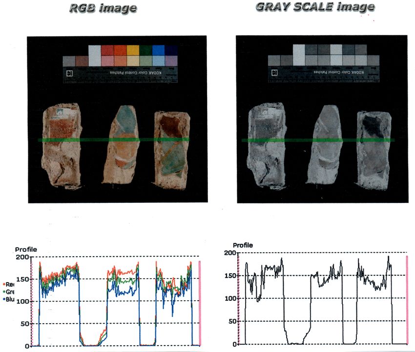
better image qualityColor images, RGB
color space
R G B
Much more on color in next lecture…
K. GraumanIssues with digital cameras
Noise
– big difference between consumer vs. SLR-style cameras
– low light is where you most notice noise
Compression
– creates artifacts except in uncompressed formats (tiff, raw)
Color
– color fringing artifacts from Bayer patterns
Blooming
– charge overflowing into neighboring pixels
In-camera processing
– oversharpening can produce halos
Interlaced vs. progressive scan video
– even/odd rows from different exposures
Are more megapixels better?
– requires higher quality lens
– noise issues
Stabilization
– compensate for camera shake (mechanical vs. electronic)
More info online, e.g.,
• http://electronics.howstuffworks.com/digital-camera.htm
• http://www.dpreview.com/Computer Other Cameras: Line Scan
Vision
Cameras
Line scanner
•The active element is 1-dimensional
•Usually employed for inspection
•They require to have
very intense light due
to small integration
time (from100msec to
1msec)Reproduced by permission, the American Society of Photogrammetry and
Remote Sensing. A.L. Nowicki, “Stereoscopy.” Manual of Photogrammetry,
Computer Thompson, Radlinski, and Speert (eds.), third edition, 1966.
Vision The Human Eye
Helmoltz’s
Schematic
EyeComputer
Vision The distribution of
rods and cones
across the retina
Reprinted from Foundations of Vision, by B. Wandell, Sinauer
Associates, Inc., (1995). Ó 1995 Sinauer Associates, Inc.
Cones in the Rods and cones in
fovea the periphery
Reprinted from Foundations of Vision, by B. Wandell, Sinauer
Associates, Inc., (1995). Ó 1995 Sinauer Associates, Inc.You can also read