Introduction to the KMA-Met Office Joint Seasonal Forecasting System and Evaluation of its Hindcast Ensemble Simulations
←
→
Page content transcription
If your browser does not render page correctly, please read the page content below
Science and Technology Infusion Climate Bulletin
NOAA’s National Weather Service
36th NOAA Annual Climate Diagnostics and Prediction Workshop
Fort Worth, TX, 3-6 October 2011

   Introduction to the KMA-Met Office Joint Seasonal Forecasting System and
                Evaluation of its Hindcast Ensemble Simulations
                           Hyun-Suk Kang, Kyung-On Boo, and ChunHo Cho
     National Institute of Meteorological Research, Korea Meteorological Administration, Seoul, Korea

1. Introduction
    Dynamical seasonal forecasts using coupled models, i.e., 1-tier approach, are now routinely made at many
operational centers in the world. For example, among twelve Global Producing Centers (GPCs) that have
contributed for providing their own real-time seasonal forecast to WMO Lead Center for Long-Range
Forecast Multi Model Ensemble (LC-LRFMME), seven centers are using coupled models while only five
centers are still based on two-tier approach. The rapid transition from two-tier to one-tier approach in seasonal
forecast are mainly caused by recent progresses in development of coupled climate models and enlargement
of understanding air-sea interactions obtained from international collaborative efforts such as TOCA program
(Wang et al., 2009). In this context, Korea Meteorological Administration (KMA), as the WMO LC-
LRFMME jointly with NOAA and one of the GPCs, is also trying to replace its operational seasonal forecast
model with a coupled model by the collaboration with U. K. Met Office.
    Recently, the GloSea4 (Global Seasonal Forecasting System version 4) of the Met Office based the
HadGEM3-AO was implemented and hindcast ensemble simulations for 14 years from 1996 to 2009 have
been accomplished. The purpose of this article is to introduce the KMA-Met Office Joint Seasonal
Forecasting system and to evaluate overall performance of its retrospective seasonal forecast particularly in
terms of predictability and skill scores. Section 2 briefly describes the joint forecast system, the model, and
design of hindcast simulations. Results of predictability and skill scores on sea surface temperature,
precipitation and surface air temperature are shown in Section 3. Finally, Section 4 summarizes the results
and further works for the operation of joint system.
2. GloSea4 and its Hindcast Simulations
2.1 GloSea4 and Joint Forecasting System
     GloSea4 is the fourth version of the Met Office seasonal ensemble prediction system based on the latest
version of HadGEM3 (Hewitt et al., 2010). It consists of the UM (Met Office Unified Model) for atmosphere,
NEMO (Nucleus for European Modeling of the Ocean) for ocean, CICE (Los Alamos sea ice model) for sea
ice, and MOSES (Met Office Surface Exchange Scheme) for land surface components with OASIS flux
coupler. The spatial resolution in the current configuration (GA 2.0) is N96L85 for atmosphere, which is
approximately 135 km in the horizontal with 85 vertical levels, and tri-polar ORCA1L75 for ocean, in which
the horizontal grid distance are 1 degree with 1/3 of a degree between 20oS and 20oN with 75 vertical levels
from the sea surface to the bottom. Details of the GloSea4 description are given in Arribas et al. (2011).
    One of the distinctive features of the GloSea4 compared to other typical seasonal forecasting system
including the current LRF system at KMA, i.e., Global Data Assimilation and Prediction System (GDAPS), is
that both the hindcast and forecast suites are run simultaneously, which allows preventing quite a burden of
resources for producing model climatology a prior to make seasonal forecast if any modification of the system
and/or bud fix is necessary. Hindcast and forecast suites are initialized with the weekly-based time cycle so
that they can update initial conditions nearly real-time, which is quite valuable to maintain consistency from
short-to-long-range forecasts. Eventually, the major benefit of KMA-Met Office joint forecasting system is to
reducing uncertainties of seasonal forecast by share ensemble members as many as possible from two centers
for both the hindcast and forecast suites. The only differences will be the initial condition for atmosphere that
______________
Correspondence to: Hyun-Suk Kang, National Institute of Meteorological Research and Korea Meteorological
Administration, Seoul, Korea; E-mail: hyunsuk306.kang@gmail.com.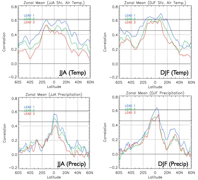
KANG ET AL. 79
comes from each center’s own 4DVAR system. At this moment, since the KMA does not have its own ocean
and sea-ice data assimilation system, initial conditions for ocean and sea-ice will be obtained from the Met
Office.
2.2 Hindcast Simulations
The ECMWF-interim reanalysis (ERA-interim) is used to initialize the atmosphere and land surface
because there is no atmospheric reanalysis available for the HadGEM3-AO. In the case of land surface
variables, an anomaly initialization approach, in which ERA-interim anomalies are calculated and then added
to the HadGEM3 model climatology, is followed to avoid the inconsistency from the very different land
surface model used in HadGEM3 and ERA-interim reanalysis. The ocean field is initialized in the same way
as in the forecast suite, i.e., the GloSea4 Ocean Data Assimilation scheme which consists of a parallel version
of the Met Office optimal interpolation scheme used for short-range ocean forecasting, except for the fact that
atmospheric fluxes to force the ODA scheme are obtained from the ERA-interim rather than from the
operational NWP system. The hindcast period is 14 years from 1996 to 2009. Initial dates are 1st, 9th, 17th,
and 25th of each month. In order to generate ensemble members by considering model uncertainties, 3
members per each initial date are generated using the stochastic kinetic energy backscatter scheme version 2
(SKEB2) (Shutts, 2005). Therefore, in total, number of 7-month-long integration of the GloSea4 system is
2,016.
3. Results
The observation dataset used for evaluation of the GloSea4 in this study are Hadley Center’s sea surface
temperature, CMAP precipitation, and ERA-interim reanalysis for the surface air temperature.
3.1 Sea Surface Temperature
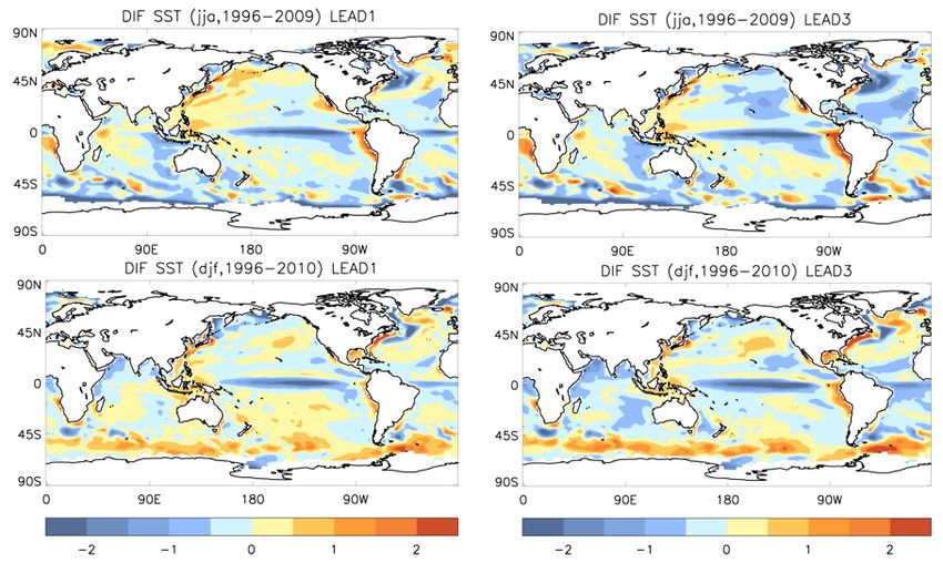
Figure 1 shows the bias of seasonal mean SST from 1-month and 3-month lead forecasts. As forecast
lead-time increases, in general, the SST bias also increases. In the results of 1-month lead forecasts, the
Fig. 1 Biases of seasonal mean SST for boreal summer (upper) and winter (lower) seasons. Left and right
panels are obtained from the results one and three months’ forecasting lead-time simulations.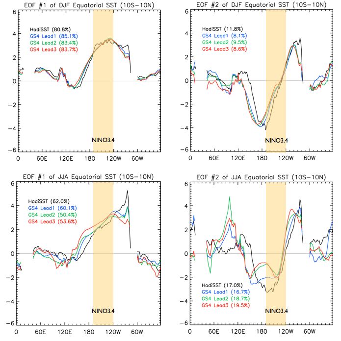
80                      SCIENCE AND TECHNOLOGY INFUSION CLIMATE BULLETIN

strongest cold bias appears along the
equatorial Pacific both for the boreal
summer and winter seasons. The spatial
pattern of SST bias seems to be somewhat
systematic, particularly in the southern
Hemisphere, which shows overall cold bias
in JJA but warm bias in DJF season.
Despite the general increase in the
amplitude of SST bias according to the
forecast leading time, its spatial structure is
fairly similar and persistent to each other.
On the contrary to the skill scores (e.g.,
bias or anomaly correlation) that indicate
the performance of the model against the
observation, signal-to-noise ratio is a
measure of predictability that implies that
how much the each ensemble member
spreads compared to ensemble mean
variance. The results of signal-to-noise
ratio show also persistent spatial patterns
with decreasing values according to the
forecast leading months (not shown). As
expected, predictability in boreal winter         Fig. 2 Correlation skill for the SST anomaly averaged over the
season is higher than in summer season                NINO3.4 area from the simulations initialized in February,
regardless to the forecast leading time.              May, August, and November.

    Anomaly correlations of the NINO3.4
SST anomalies for the four different initial
months are shown in Figure 2. Each month
has 12 ensemble members with time-
lagged initial dates and SKEB2 physics.
Overall, skill scores for NINO3.4 index are
higher in cold season than in warm season.
The skill score drops rapidly from April to
July from the simulations initialized on
February and November, which is
associated limitation of predictability of
SST during the spring time, called “spring
barrier”. The spring barrier issue is one of
the common problematic features in
coupled GCM, and suspected to be
associated with failure of surface wind
stress over the equatorial Pacific. It is
interesting to note skill score for the JJA
forecast is relatively lower than other
seasons in the beginning of the forecast,
however; the score remains with persistent
and relatively higher values for the longer
forecast lead-time. The red lines in Figure
2 denote the score calculated from the Fig. 3 The first (left panel) and second (right panel) leading EOF
ensemble mean, and black solid, dashed       modes for the SSTA averaged over 10S-10N. Black, blue,
and dotted lines are average, maximum and    green, and red lines indicate observation, GS4 results with one,
                                             two, and three month lead time, respectively.
minimum values from each individual
KANG ET AL. 81
ensemble members. It is clearly recognized that scores from the ensemble mean are quite close to the
maximum scores of individual member, or in some cases, it is superior to maximum of individual ensemble
members.
In order to investigate SST
variability, EOF analysis was conducted
for the SST anomaly against the
latitudinal mean between 10oS~10oN
(Fig. 3). During the boreal summer (JJA),
the observed leading mode represents a
peak SSTA in the Nino 3 region rather
than 3.4 region (lower left in Fig. 3).
Meanwhile, that of boreal winter (DJF)
is apparent in somewhat wide areas
including both the Nino3.4 and Nino 3
areas. Those patterns of leading mode of
SSTA along the equator are captured
pretty well by the GloSea4. In JJA, the
variability of SST over central Pacific
tends to be overestimated by the
GloSea4, which are getting stronger to
the longer forecast lead-time. From the
second leading mode during DJF season,
the area of strong variability extends
westward in results from the GS4 Fig. 4 Anomaly correlation of surface air temperature (upper) and
compared to the observation. precipitation (lower) for JJA (left panel) and DJF (right panel).
Blue, green, and red lines indicate one, two and three months’
3.2 Precipitation and Surface Air forecast leads.
Temperature
Since the hindcast period of the GloSea4 is somewhat short (only 14 years), the corresponding correlation
value with 0.05 and 0.01 significance levels are somewhat higher which are about 0.45 and 0.61, respectively.
As like in other coupled seasonal forecasting system, significant anomaly correlation scores for the surface air
temperature and precipitation are concentrated mainly over tropical regional about between 20oS-20oN (Fig.
4). It is clear that anomaly correlation scores are decreasing rapidly in accordance with the forecast leading
month. East Asia region, in which the skill scores are quite low as in other extra-tropical areas, meaningful
scores with 0.05 significance levels are limited only spring and autumn seasons surface air temperature in
cases of less than three months’ forecast leading time (not shown). Nevertheless, in terms of practical sense of
seasonal forecast, it is promising to note that biases of surface air temperature and precipitation over East Asia
are quite systematic and persistent as a function of forecast leading months.
4. Summary and Further Works
In this study, overall skill of the GloSea4 system, which will be operated as an operational seasonal
forecasting system at KMA and joint system between KMA and Met Office, have been examined. The skill
scores obtained from hindcast ensemble simulations seem to be comparable against with other coupled
climate models. However, it should be carefully investigated within intercomparison framework to find out
strength and weakness of the GloSea4. Robust evaluation of hindcast ensemble runs including the Asian
monsoon, sub-seasonal variability such as MJO and their impacts over Asia should be further investigated. In
addition, horizontal resolution both for the atmosphere and ocean will be increased a prior to the operation up
to N216 (~ 60 km) and quarter degrees (in extra-tropical region), respectively.
Acknowledgements. This study was supported by the Grant NIMR-2011-B-2. The authors are grateful for
the Met Office colleagues, Drs. A. Arribas and C. MacLachlan for their providing successful implementation
of the GloSea4 to the KMA.82 SCIENCE AND TECHNOLOGY INFUSION CLIMATE BULLETIN
References
Arribas, A., M. Glover, A. Maidens, K. Peterson, M. Gordon, C. MacLachlan, R. Graham, D. Fereday, J.
Camp, A. A. Scaife, P. Xavier, P. McLean, A Colman, and S. Cusack, 2011, The GloSea4 Ensemble
Prediction system fore seasonal forecasting, Mon. Wea. Rev., 139, 1891-1910.
Hewitt, H. T., D. Copsey, I. D. Culverwell, C. M. Harris, R. S. R. Hill, A. B. Keen, A. J. McLaren, and E. C.
Hunke, 2010, Design and implementation of the infrastructure of HadGEM3: The next generation Met
Office climate modeling system. Geosci. Model Dev. Discuss., 3, 1861-1937.
Shutts, G., 2005: A kinetic energy backscatter algorithm for use in ensemble prediction systems. Quart. J.
Roy. Meteor. Soc., 131, 3079-3102.
Wang, B. and co-authors, 2009: Advance and prospectus of seasonal prediction: Assessment of the
APCC/CliPAS 14-model ensemble retrospective seasonal prediction (1980-2004), Clim. Dyn., 33, 93-117.You can also read