NP Bayes Functional Regression for a PK/PD Semi-Mechanistic Model: A talk for advertisement and discussion
←
→
Page content transcription
If your browser does not render page correctly, please read the page content below
NP Bayes Functional Regression for a PK/PD
         Semi-Mechanistic Model:
  A talk for advertisement and discussion

                     Michele Guindani
(joint work with Peter Müller, Gary Rosner and L. Friberg)

                  Department of Biostatistics
                UT MD Anderson Cancer Center

                 SAMSI, Wed 14th, 2010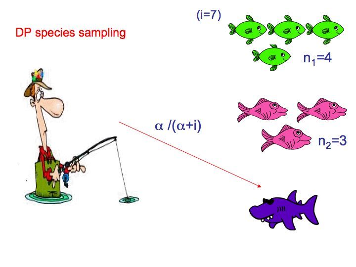
Outline
¬ Semi-mechanistic PK/PD models
Bayesian joint PK/PD modeling
® The advantage of a Non-parametric (NP) Bayesian Approach
¯ A pair of plots to prove we can do things.
¯ Discussion, problems, issues þ things to work on!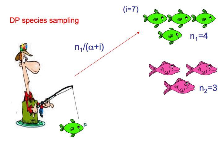
¬ Semimechanistic PK/PD models: what are those? Bayesian joint PK/PD Modeling ® Non-parametric (NP) Bayes ¯ We can do things!
PK/PD from the perspective of a dummy statistician

    + Population Pharmacokinetics (PK) studies the behavior of a
      drug in the body over a period of time (absorption,
      distribution, metabolism, excretion).

       Often, we say that PK is the study of what the body does to
       a drug.

    þ Plays a pivotal role in direct patient care for the construction
      of patient dosing strategies.
PK Time Concentration profiles
GOAL: quantitatively assess some typical pharmacokinetic
parameters, upon observation/estimation of the individual plasma
concentration profiles over time
Source:Wikipedia!Data
ý Data usually follow a precise administration/measurement
schedule.
For example, in one of the studies reported in Friberg et al,
2002, data are from 45 patients with different cancer forms,
who received paclitaxel in a total of 196 cycles (varying
between one and 18 cycles per patient; median, three cycles),
were analyzed.
Paclitaxel was administered as a 3-hour infusion, with an
initial dose of 175 mg/m2 every 3rd week. Dose adjustments
were guided by hematological and nonhematological toxicity,
which resulted in a final dose range of 110 to 232 mg/m2.
Plasma concentrations were monitored on course 1 and course
3, with an average of 3.5 samples per patient and course.PK model
ý Typically, the PK models try to artificially “replicate” what
happens to the drug once in the body.
ý Graphically, we can represent a simple model as follows (from
AdaptGuide)
This is described as a linear two-compartment model. In our
application, we use it for modeling the unbound plasma
concentrations of paclitaxel.ý Mathematically, the response (concentration) in a sample of
individuals is assumed to reflect both measurement error and
intersubject variability,
K
yij = fij (θiK , xij ) + εij , i = 1, . . . , N, j = 1, . . . , ni ,
where fij (θiK , xij ) is a function for predicting the jth response
in subject i, θi is a vector of individual PK parameters and xij
is a vector of known quantities or covariates.
k denotes the observed concentration for individual i at
Here yij
time j, or Ci (tj ).A system of ODE for the PK
ý The graphical scheme shown above represents systematically the
following system of differential equations
CL CLd CLd
dxc (t)
=− + xc (t) + xp (t) + r(t)
dt Vc Vc Vp
dxp (t) CL CLd
= c xc (t) − p xp (t)
dt V V
xc (t)
C(t) = c
V
where CL is the system clearance, V c and V p are the volumes of
distribution of the central and peripheral compartment, CLp is the
intercompartmental clearance and r(t) is the rate of infusion into
the first compartment.
I C(t) þ time course of the unbound plasma concentrations.A system of ODE for the PK
ý The system of linear ODEs for PK modeling is “doable”: it can be
estimated with non linear least square techniques (ODE solver - but
see Paolo Vicini’s and Lang Li’s talks yesterday - we need
prior/penalty terms to enforce identifiability).
ý PK modelers most often assume that
θi = g(φ, xi ) + ηi
where φ is a vector of population parameters, xi is a vector of
known individual specific covariates (held constant across cycles)
and ηi is the individual random effect.
Estimation is done through non linear mixed effects models and
related algorithms. For example, in NONMEM the mixed effect
model is linearized by using the first order Taylor series expansion
with respect to ηi (and εij ). (check S. Gosh, R. Leary, P. Vicini)A system of ODE for the PK
ý The system of linear ODEs for PK modeling is “doable”: it can be
estimated with non linear least square techniques (ODE solver - but
see Paolo Vicini’s and Lang Li’s talks yesterday - we need
prior/penalty terms to enforce identifiability).
ý PK modelers most often assume that
θi = g(φ, xi ) + ηi
where φ is a vector of population parameters, xi is a vector of
known individual specific covariates (held constant across cycles)
and ηi is the individual random effect.
Estimation is done through non linear mixed effects models and
related algorithms. For example, in NONMEM the mixed effect
model is linearized by using the first order Taylor series expansion
with respect to ηi (and εij ). (check S. Gosh, R. Leary, P. Vicini)Dependence on Covariates
ü The PK model is often completed by equations, relating specific
covariates to the parameters of the model; for example,
log CL =β1 + β2 × (BSA) + β3 × (BIL)
log V c =β4 + β5 × (BSA)
log V p =β6 + β7 × (BSA),
where BSA is the body surface area and BIL is bilirubin
(hematoidin, excreted in bile).
For each subject i,
θiP K = (β1,i , β2,i , β3,i , β4,i , β5,i , β6,i , β7,i , CLpi )Dependence on Covariates
ü The PK model is often completed by equations, relating specific
covariates to the parameters of the model; for example,
log CL =β1 + β2 × (BSA) + β3 × (BIL)
log V c =β4 + β5 × (BSA)
log V p =β6 + β7 × (BSA),
where BSA is the body surface area and BIL is bilirubin
(hematoidin, excreted in bile).
For each subject i,
θiP K = (β1,i , β2,i , β3,i , β4,i , β5,i , β6,i , β7,i , CLpi )Pharmacodynamics
+ Pharmacodynamics (PD) refers to the time-course and
intensity of drug action or response.
We can say that PD studies what a drug does to the body.
+ The pharmacologic response depends on the drug binding to
its target. Receptors determine the quantitative relationship
between drug dose and pharmacologic effect. The
concentration of the drug at the receptor site influences the
drug’s effect. Hence, PK and PD are inherently related.+ Joint kinetic–dynamic modeling is important to predict how
drug concentration affects the response.
ý GOAL: Establish relationships between drug
concentrations and individual responses (e.g, in terms
of myelosuppression)
þ produce therapeutic benefits while minimizing
side-effects
þ find Optimal Dose/Administration schedule
“The major challenge for health care professionals involved in
clinical psychopharmacology is to understand and compensate for
individual variations in drug response” (Greenblat et. al
-Psychopharmacology -the Fourth Generation of Progress).+ Joint kinetic–dynamic modeling is important to predict how
drug concentration affects the response.
ý GOAL: Establish relationships between drug
concentrations and individual responses (e.g, in terms
of myelosuppression)
þ produce therapeutic benefits while minimizing
side-effects
þ find Optimal Dose/Administration schedule
“The major challenge for health care professionals involved in
clinical psychopharmacology is to understand and compensate for
individual variations in drug response” (Greenblat et. al
-Psychopharmacology -the Fourth Generation of Progress).Empirical and Mechanistic Dose/Response models
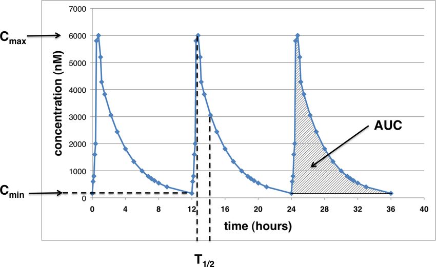
+ Empirical Dose/Response models relate drug exposure (AUC,
time above threshold) of anticancer drugs to some measure of
the drug’s effect, such as the nadir of leukopenia or surviving
fraction of leukocytes at nadir
+ The Emax model is a common descriptor of dose–response
relationships,
Emax C
E=
EC50 + C
where Emax is the maximum response of the system to the
drug and EC50 is that concentration of drug producing 50% of
Emax .Physiology based Semi-Mechanistic (SM) PK/PD models
+ Physiology based models with parameters that refer to actual
processes and conditions may be preferable.
Ideal physiology-based models separate system parameters,
common across drugs, from drug–specific parameters.
4 SM PK/PD models describe the entire course of the response
profile (e.g., leukopenia) by using the entire time course of
plasma concentration as input.
(e.g. Minami et al., 1998, 2001, Friberg et al. 2000, 2002,
2003)PD model
For example, Friberg et al. (2002) develop a structural model
for myelosupression consisting of
¬ One compartment representing stem cells and progenitor cells
(i.e. Proliferative cells, sensitive to drugs – Prol)
Three transit compartments with maturing cells (– Transit)
® A compartment of circulating observed blood cells (– Circ)PD model
o The model consists of a system of non-linear differential equations
(Friberg, 2002)
γ
Circ0
dP rol/dt = kprol P rol (1 − Edrug ) − ktr P rol
Circ
dT ransit1 /dt = ktr P rol − ktr T ransit1
dT ransit2 /dt = ktr T ransit1 − ktr T ransit2
dT ransit3 /dt = ktr T ransit2 − ktr T ransit3
dCirc/dt = ktr T ransit3 − ktr Circ
The effect of the PK component on the PD model is captured by a
term like
Edrugs = Sl × C(t) or an Emax model
θiP D = (Circ0,i , γi , ktr,i , Sli )PD model
o Hence, the model explicitly separate between system parameters...
• mean transit time: M T T = (n + 1)/ktr where n is the number of
transit compartments
• baseline: Circ0
• feedback: γ
• ..and drug specific parameters: Sl or Emax , and EC50
The feedback was necessary to describe the rebound of cells
(overshoot compared with the baseline value Circ0 ). The
proliferation rate can be affected by endogenous growth factors and
the G-CSF levels increase when the neutrophil counts are low.Data
+ The collection of data on the response effect doesn’t seem to
be as systematic as in the case of the measurements of drug
concentration.
+ In order to fit the solution of the previous system of ODE’s by
non-linear least square techniques, we typically need more and
well spaced points.
14
12
●
●
10
●
ANC
8
6
4
●
0 200 400 600 800
timeData
+ The collection of data on the response effect doesn’t seem to
be as systematic as in the case of the measurements of drug
concentration.
+ In order to fit the solution of the previous system of ODE’s by
non-linear least square techniques, we typically need more and
well spaced points.
9
8
7
6
ANC
5
●
4
3
2
0 200 400 600 800
timeData
+ The collection of data on the response effect doesn’t seem to
be as systematic as in the case of the measurements of drug
concentration.
+ In order to fit the solution of the previous system of ODE’s by
non-linear least square techniques, we typically need more and
well spaced points.
12
11
10
ANC
9
8
●
7
●
6
0 200 400 600 800
●
timeData
+ The collection of data on the response effect doesn’t seem to
be as systematic as in the case of the measurements of drug
concentration.
+ In order to fit the solution of the previous system of ODE’s by
non-linear least square techniques, we typically need more and
well spaced points.
●
15
10
ANC
5
●
0
0 200 400 600 800
time¬ Semimechanistic PK/PD models: what are those? Bayesian joint PK/PD Modeling ® Non-parametric (NP) Bayes ¯ We can do things!
Bayesian Approach

    o ADVANTAGES:

    • The Bayesian approach allows incorporation of prior
      information (e.g. from existing literature)

    • There are no hidden assumptions: priors make us honest!

    • Inference on the parameters of interest is summarized in a
      posterior distribution, with proper assessment of the
      estimation uncertainty.

    • The estimation of the PK/PD parameters can be obtained
      simultaneously.
Bayesian Approach
o DATA: concentration and ANC measurements for
i = 1, . . . , N patients
C (t) = f P K (θiP K ) + εi
i
Circi (t) = f P D (θiP K , θiP D ) + ηi
with εi ∼ N (0, σ12 ) ηi ∼ N (0, σ22 )
θi = (θiP K , θiP D )∼ N (Θ, Σ)
π(σ1 ) π(σ2 ) π(Θ) π(Σ)Comments related to yesterday’s talks
þ It’s possible to incorporate covariate information, e.g. by
assuming
θiP K ∼ N (βiK Xi , ΣK
i )
þ Prior elicitation and prior regularization are important issues,
although here I am not concentrating on those - see Johnson’s
and Thall’s talks yesterday on prior choice.Bayesian Approach
o PK models:
Gelman et al (1996)
Stroud et al (2001)
Winbugs implementations:
Lunn et al (2002)
Winbugs + Full PK/PD model
Kathman et al (2007)
ý Clustering of the patient specific time courses may help
improve the assessment of the optimal dose for anticancer
treatmentsAn argument for Clustering
ý MLE estimates for the PD model
14
6
12
5
10
●
4
ANC patient 3
ANC patient 7
8
3
6
●
●
4
●
2
●
●
2
● ●
●
1
●
●
● ● ●
0
0 200 400 600 800 1000 0 200 400 600 800 1000
time time
o The different shapes may
5
●
●
suggest clustering of
4
●
patients’ profiles
ANC patient 14
3
2
●
1
●
●
ý NP Bayes Approach
0 200 ● 400 600 800 1000
time¬ Semimechanistic PK/PD models: what are those? Bayesian joint PK/PD Modeling ® Non-parametric (NP) Bayes ¯ We can do things!
NP Bayes: DP Model
  NP Bayes model: Our prior probability is also considered
     “uncertain”,

                        θ | G ∼ G(θ),   G ∼ P (G).

    • One of the most used NP prior is the DP prior.
    • Many alternative definitions are possible (check P. Mueller
      (alias W. Johnson)’s talk on Monday).
      For example,
                                   X∞
                          G(·) =       pk δθk∗ (·),
                                    k=1
               i.i.d.                   Qk−1
      where θk∗ ∼ G∗ , and pk = qk        i=1 (1   − qi ), qi ∼ Beta(1, α),

                             ï G ∼ DP (α, G∗ ),
NP Bayes: DP Model
NP Bayes model: Our prior probability is also considered
“uncertain”,
θ | G ∼ G(θ), G ∼ P (G).
• One of the most used NP prior is the DP prior.
• Many alternative definitions are possible (check P. Mueller
(alias W. Johnson)’s talk on Monday).
For example,
X∞
G(·) = pk δθk∗ (·),
k=1
i.i.d. Qk−1
where θk∗ ∼ G∗ , and pk = qk i=1 (1 − qi ), qi ∼ Beta(1, α),
ï G ∼ DP (α, G∗ ),NP Bayes: DP Model
Some properties.
I E(G) = G∗ and α is called the mass or precision parameter.
I G is discrete ï positive probability of ties of θi ’s.
ï Clustering
I Predictive distribution (a.k.a. Chinese restaurant process
or species sampling characterization.)Unsupervised model-based clustering
NP Bayes Approach
o In the previous Bayesian model, we substitute the NP
specification
C (t) = f P K (θiP K ) + εi
i
Circi (t) = f P D (θiP K , θiP D ) + ηi
with εi ∼ N (0, σ12 ) ηi ∼ N (0, σ22 )
θi = (θiP K , θiP D )|G∼ G
G∼ DP (α, G0 )
G0 ≡ N (Θ, Σ)
π(σ1 ) π(σ2 ) π(Θ) π(Σ)GOAL:
o We want to provide a coherent probability model that tries to
address the previously mentioned challenge:
“The major challenge for health care professionals involved in
clinical psychopharmacology is to understand and compensate
for individual variations in drug response”
þ Cluster the patients according to their PK/PD profiles
þ Predict an individual PD profiles on the basis of its PK profile
(or PK parameters)
þ This is achieved by joint modeling of the PK and PD curves
and joint inference on the vector parameter θi (þ check back
Dunson’s talk on Monday)Some Issues and Challenges
5 We can model the ODE’s parameters with a DP þ use an
MCMC algorithm þ describe the full time course of the PK
and PD and obtain inference on between and within subject
variability (inter-occasion/inter-individual).
5 A full, complete, MCMC requires solving the systems of
ODE’s at each iteration ý it can be slow and painful !!
5 The system of ODE’s for the PD model is non-linear and
highly unstable (especially if we have just a few data!)
5 The likelihood is presumably extremely multimodal
A possibility: use some approximation of the likelihood; for
example we could linearize around the value of the MLE
estimates.Some Issues and Challenges
5 We can model the ODE’s parameters with a DP þ use an
MCMC algorithm þ describe the full time course of the PK
and PD and obtain inference on between and within subject
variability (inter-occasion/inter-individual).
5 A full, complete, MCMC requires solving the systems of
ODE’s at each iteration ý it can be slow and painful !!
5 The system of ODE’s for the PD model is non-linear and
highly unstable (especially if we have just a few data!)
5 The likelihood is presumably extremely multimodal
A possibility: use some approximation of the likelihood; for
example we could linearize around the value of the MLE
estimates.Gaussian approximation around the MLE’s
θ̂iK |βiK , Xi ∼ N (βiK Xi , Σ̂ki )
θ̂iD | θiK , βiK , Xi , θiD ∼ N (Ĥi (βiK Xi − θ̂iK ) + θiD , Σ̂D
i )
where θ̂iK , θ̂iD are the MLE estimates and Σ̂ki , Σ̂D
i the
corresponding (marginal and conditional) covariance matrices.
The model is completed by assigning appropriate priors to the
parameters of interest; in particular,
θi = (vec(βiP K ), θiP D )|G∼ G
G∼ DP (α, G0 )
G0 ∼ NP K (β0 , ∆β ) × NP D|P K (θ0D , ∆D
0 )Gaussian approximation around the MLE’s
θ̂iK |βiK , Xi ∼ N (βiK Xi , Σ̂ki )
θ̂iD | θiK , βiK , Xi , θiD ∼ N (Ĥi (βiK Xi − θ̂iK ) + θiD , Σ̂D
i )
where θ̂iK , θ̂iD are the MLE estimates and Σ̂ki , Σ̂D
i the
corresponding (marginal and conditional) covariance matrices.
The model is completed by assigning appropriate priors to the
parameters of interest; in particular,
θi = (vec(βiP K ), θiP D )|G∼ G
G∼ DP (α, G0 )
G0 ∼ NP K (β0 , ∆β ) × NP D|P K (θ0D , ∆D
0 )¬ Semimechanistic PK/PD models: what are those? Bayesian joint PK/PD Modeling ® Non-parametric (NP) Bayes ¯ We can do things!
Some plots.
    o Clustering of the MLE estimates

                 250
                 200
                 150
                 100
                 50
                 0

                       3   4            5           6              7   8

                               # clusters across MCMC iterations
Predictive inference.
o We observe only the concentration profile for some patients
and want to predict their PD profile
●
6
5
●
4
Concentration
●
3
●
●
2
1
●
●
●
●
● ●
0
0 10 20 30 40 50
timePredictive inference.
o Predicted PD profile and comparison with actual (known) data
6
●
ANC patient 7
4
●
2
●
● ●
● ●
0
0 100 200 300 400 500 600 700
timeConclusions/Discussion
o We can provide a coherent probability model for the analysis
of PK/PD mechanistic models.
o By using a NP bayes approach, we obtain inference on
patients’ clustering according to their concentration/response
profiles.
o Eventually, the clustering specification will allow the
prediction of new patients’ PD profiles on the basis of PK
profiles (and/or other covariate information)
o Many challenges and opportunities, connected to the nature
and availability of the data, the depth of knowledge of the
individual PK/PD dynamics, the NP machinery we use ad the
concrete applications.You can also read