Joint Summarization of Large-scale Collections of Web Images and Videos for Storyline Reconstruction
←
→
Page content transcription
If your browser does not render page correctly, please read the page content below
Joint Summarization of Large-scale Collections of Web Images and Videos
                          for Storyline Reconstruction

            Gunhee Kim                                 Leonid Sigal                                Eric P. Xing
     Disney Research Pittsburgh                 Disney Research Pittsburgh                  Carnegie Mellon University
           gunhee@cs.cmu.edu                   lsigal@disneyresearch.com                          epxing@cs.cmu.edu

                         Abstract

    In this paper, we address the problem of jointly sum-
marizing large sets of Flickr images and YouTube videos.
Starting from the intuition that the characteristics of the
two media types are different yet complementary, we de-
velop a fast and easily-parallelizable approach for creating
not only high-quality video summaries but also novel struc-
tural summaries of online images as storyline graphs. The
storyline graphs can illustrate various events or activities
associated with the topic in a form of a branching network.
The video summarization is achieved by diversity ranking
on the similarity graphs between images and video frames.
The reconstruction of storyline graphs is formulated as the
inference of sparse time-varying directed graphs from a set
of photo streams with assistance of videos. For evaluation,
we collect the datasets of 20 outdoor activities, consisting
of 2.7M Flickr images and 16K YouTube videos. Due to the
large-scale nature of our problem, we evaluate our algo-
rithm via crowdsourcing using Amazon Mechanical Turk.
In our experiments, we demonstrate that the proposed joint
summarization approach outperforms other baselines and                Figure 1. Benefits of jointly summarizing Flickr images and
our own methods using videos or images only.                          YouTube videos illustrated on a fly+fishing activity. (a) Although
                                                                      images in a photo stream are taken consecutively, the underlying
                                                                      sequential structure between images is missing, which can be dis-
1. Introduction                                                       covered with the help of a collection of videos. (b) Typical user
                                                                      videos contain noisy and redundant information, which can be re-
   The recent explosive growth of online multimedia data              moved using similarity votes cast by a large set of images that
has posed a new set of challenges in computer vision re-              are taken more carefully from canonical viewpoints. The frames
search. One of such infamous difficulties is that much of the         within red boxes are selected as video summary using our method.
data accessible to users are neither refined nor structured for
later use, and subsequently has led to the information over-          camcorders. For example, any smartphone user can seam-
load problem; users are often overwhelmed by the flood of             lessly record the memorable moments via both photos and
unstructured pictures and videos. Therefore, it is increas-           videos by switching between the two modes with a tap.
ingly important to automatically summarize a large set of                More importantly, jointly summarizing images and
multimedia data in an efficient yet comprehensive way.                videos is mutually-rewarding for the summarization pur-
   In this paper, we address the problem of joint summa-              pose, because their characteristics as recording media are
rization of large sets of online images (e.g. Flickr) and             different yet complementary (See Fig.1). The strength of
videos (e.g. YouTube), particularly in terms of storylines.           images over videos lies in that images are more carefully
Handling both still images and videos is becoming neces-              taken so that they capture the subjects from canonical view-
sary, due to the recent convergence between cameras and               points in a more semantically meaningful way. However,

                                                                  1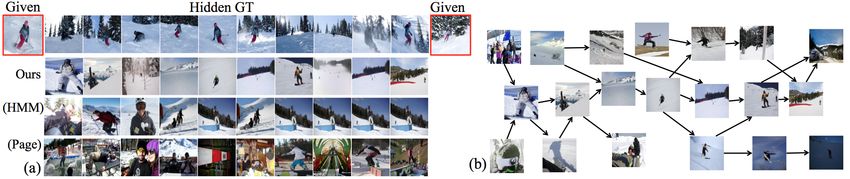
still images are fragmentally recorded, and thus the sequen-      1.1. Previous work
tial structure is often missing even between consecutive im-          Here we overview representative literature from three
ages in a single photo stream. On the other hand, videos          lines of research that are related to our work.
are motion pictures, which convey temporal smoothness be-
                                                                      Structured image summarization. One of most tradi-
tween frames. However, one major issue with videos is that
                                                                  tional ways to summarize image databases is the image re-
they contain redundant and/or noisy information with, of-
                                                                  trieval that returns a small number of representative images
ten, poor quality, such as backlit subjects, motion blurs,
                                                                  with ranking scores for a given topic (e.g. Google/Bing im-
overexposure, and full of trivial backgrounds like sky or wa-
                                                                  age search engines). Recently, there have been several im-
ter. Therefore, as shown in Fig.1, we take advantage of sets
                                                                  portant threads of image summarization work in computer
of images to get rid of such noisy, redundant, or semanti-
                                                                  vision as follows. The first notable direction is to orga-
cally meaningless parts of videos. In the reverse direction,
                                                                  nize image databases with structural visual concepts such as
we leverage sets of videos to glue fragmented images into
                                                                  WordNet hierarchy [5] or word dictionaries [21]. Another
coherent and smooth threads of storylines.
                                                                  line of work is to organize visitors’ unstructured commu-
    We first collect large sets of photo streams from Flickr      nity photos of popular landmarks in a spatially browsable
and user videos from YouTube for a topic of interest (e.g.        way [18]. However, the concept of stories has not been ex-
fly+fishing). We summarize each video with a small set of         plored much for structured image summarization yet. The
keyframes using similarity votes cast by the images from          work of [9] is related to our work in that it leverages Flickr
the most similar photo streams. Subsequently, leveraging          images and its objective is motivated by the photo story-
the continuity information between the selected keyframes         line reconstruction. However, [9] is a preliminary research
in videos, we discover the underlying sequential structure        that solely focuses on alignment and segmentation of photo
between images in each photo stream, and summarize the            streams; no storyline reconstruction is explored.
sets of photo streams in the form of storyline graphs. We             Story-based video summarization. The story-based
represent the storylines as directed graphs in which the ver-     video summary has been actively studied in the context of
tices correspond to dominant image clusters, and the edges        sports [7] and news [15]. However, in such applications, the
connect the vertices that sequentially recur in many photo        videos of interest usually contain a small number of spec-
streams and videos. The summarization in the form of sto-         ified actors in fixed scenes with synchronized voices and
ryline graphs is advantageous especially for the topics that      captions, all of which are not available in unstructured user
consist of a sequence of activities or events repeated across     images and videos on the Web. The work of [8] may be
the photo and video sets, such as recreational activities, hol-   one of the closest to our work, because images are used
idays, and sports events. Moreover, the storyline graphs can      as a prior to create semantically-meaningful summaries of
characterize various branching narrative structures associ-       user-generated videos on eBay sites. The key difference of
ated with the topic, which help users understand the under-       our work is that we complete a loop between jointly sum-
lying big picture surrounding the topic (e.g. activities that     marizing images and videos in a mutually-rewarding way.
people usually enjoy during their fly+fishing trips).             Also, our storyline summaries can support multiple branch-
    In our approach, the video summarization is achieved by       ing structures unlike simple keyframe summaries of [8].
diversity ranking on the similarity graphs between images         Lately, the summarization of ecocentric videos [12, 13] has
and video frames (section 3). The reconstruction of story-        emerged as an interesting topic, in which compact story-
line graphs is formulated as the inference of sparse time-        based summaries are produced from user-centric daylife
varying directed graphs from a set of directed trees created      videos. The objective of our work differs in that we are in-
from photo streams with assistance of videos (section 4).         terested in the collections of online images and videos that
As a result, our method provides several appealing proper-        are independently taken by multiple anonymous users, in-
ties, especially for large-scale problems, such as optimality     stead of a single user’s hours-long videos.
guarantee, linear complexity, and easy parallelization.               Computer vision leveraging both images and videos.
    For evaluation, we collect the datasets of 20 outdoor         Recently, it is gaining popularity to address challenging
recreational activities, which consist of about 2.7M images       computer vision problems by leveraging both images and
of 35K photo streams from Flickr and 16K videos from              videos. New powerful algorithms have been developed
YouTube. Due to the large-scale nature of our problems,           by pursuing synergic interplay between the two comple-
we evaluate our algorithms via crowdsourcing using Ama-           mentary domains of information, especially in the areas of
zon Mechanical Turk (section 5). In our experiments, we           adapting object detectors between images and videos [16,
quantitatively show that the proposed joint summarization         20], human activity recognition [3], and event detection [4].
approach outperforms other baselines and our method using         However, the storyline reconstruction extracted from both
videos or images only, for the both tasks of video summa-         images and videos still remains as a novel and largely
rization and storyline reconstruction.                            under-addressed problem.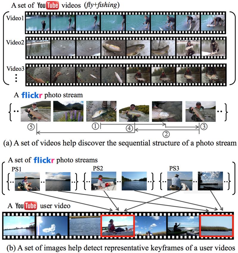
1.2. Summary of Contributions                                        resized image. For similarity measure σ, we use histogram
   We summarize the contributions of this work as follows.           intersection. The three descriptors are equally weighted.
   (1) We propose an approach to jointly summarize large                K-NN graphs between photo streams and videos. Due
sets of online images and videos in a mutually-rewarding             to the extreme diversity of the Web images and videos as-
way. Our method creates not only high-quality video sum-             sociated even with the same keyword, we build K-nearest
mary but also a novel structural summary of online images            graphs between P and V so that only sufficiently similar
as storyline graphs, which can visualize various events and          photo streams and videos help summarize one another.
activities associated with the topic in a form of branching             For each photo stream P l ∈ P, we find KP -nearest
networks. To the best of our knowledge, our work is the first        videos calculating the similarity by Naive-Bayes Nearest-
attempt so far to leverage both online images and videos for         Neighbor method [2] as follows. For all pairs of photo
building of storyline graphs.                                        stream P l and videos V n ∈ V, we obtain the first near-
   (2) We develop algorithms for video summarization and             est neighbor in V n of each image p ∈ P l , denoted by
storyline reconstruction, properly addressing several key            NN(p).    The similarity from P l to V n is computed by
                                                                                             2                               l
                                                                     P
challenges of related large-scale problems, including opti-             p∈P l kσ(p, NN(p))k . As results, we can find N (P ) as
mality guarantees, linear complexity, and easy paralleliza-          the KP -nearest videos to P l . We set Kp = c · log(|V|)
tion. With experiments on large-scale Flickr and YouTube             with c = 1. Likewise, we run the same procedure to obtain
datasets and crowdsourcing evaluations through Amazon                KV -nearest photo streams N (V n ) for each video V n .
Mechanical Turk, we show the superiority of our approach                Since we leverage sufficiently large image/video datasets
over competing methods for both summarization tasks.                 that reasonably well cover each topic, we observe that the
                                                                     domain difference between images and videos does not af-
2. Problem Setting                                                   fect performance much. For example, when we find out K
      Input. The input is a set of photo streams P =                 nearest images to a video frame from our image dataset, the
{P 1 , · · · , P L } and a set of videos V = {V 1 , · · · , V N },   matched frame and images tend to be similar to one another.
for a topic class of interest. L and N indicate the num-
ber of input photo streams and videos, respectively. Each            3. Video Summarization
photo stream, denoted by P l = {pl1 , · · · , plLl }, is a set of        The summarization of each video V n ∈ V runs as fol-
photos taken in sequence by a single photographer within             lows. We first build a similarity graph GVn = (X n , E n )
a fixed period of time [0, T ], single day in this paper. We         where the node set is the frames in V n and the images of its
assume that each image pli is associated with a timestamp            neighbor photo streams N (V n ) (i.e. X n = V n ∪ N (V n )),
tli , and images in each photo stream are temporally ordered.        and the edge set consists of two groups: E n = EIn ∪ EO n
                                                                                                                               . EIn
We uniformly sample each video into a set of frames every            is the edge set between the frames within V n , in which con-
0.5 sec, which is denoted by V n = {v1n , · · · , vN n
                                                       n }. As a     secutive frames are connected as k-th order Markov chain,
notational convention, we use superscripts to denote photo           and the weights are computed by feature similarity. EO   n
                                                                                                                                 de-
streams/videos and subscripts to denote images/frames.               fines the edges between frames in V n and the images of
      Output. The output of our algorithm is two-fold. The           N (V n ). More specifically, each image in N (V n ) casts
first output is the summary S n of each video V n ∈ V (i.e.          similarity votes by connecting with its kP -nearest frames
S n ⊂ V n ). We pursue keyframe-based summarization (e.g.            with the weight of feature similarity. Since most images
[8]), in which S n is chosen as ν n number of most represen-         shared online are carefully taken by photographers who try
tative but discriminative keyframes out of V n . Its technical       to express their intents to be as clear as possible, even sim-
details will be discussed in Section 3. The second output is         ple similarity voting by a crowd of such images can dis-
the storyline graphs G = (O, E). The vertices O correspond           cover high-quality and semantically-meaningful keyframes,
to dominant image clusters across the dataset, and the edge          which will be demonstrated in the experiments (Section 5).
set E connects the vertices that sequentially recur in many              Once we build the graph GVn = (X n , E n ), we select ν n
photo streams and videos. More rigorous mathematical def-            keyframes as a summary of V n using the diversity rank-
inition will be given in Section 4.                                  ing algorithm proposed in [10], which is formulated as a
      Image Description and Similarity Measure. We ap-               temperature maximization by placing ν n number of heat
ply three different feature extraction methods to images and         sources in V n . Intuitively, the sources should be located
frames of videos. We densely extract HSV color SIFT and              in the nodes that are densely connected to other nodes with
histogram of oriented edge (HOG) feature on a regular grid           high edge weights. At the same time, the sources should be
of each image and frame at steps of 4 and 8 pixels, respec-          sufficiently distant from one another because nearby nodes
tively. We build an L1 -normalized three-level spatial pyra-         to the sources will already have high temperatures. We let
mid histogram for each feature type. Finally, we obtain the          Gn be the adjacency matrix of GVn . In order to model the
Tiny image feature [21], which is RGB values of a 32×32              heat dissipation, a ground node g is connected to all nodes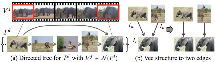
with a constant dissipation conductance z (i.e. appending
an |Gn | × 1 column z to the end of Gn ). The optimization
of ν n keyframe selection can be expressed by
        X
max          u(x)                                      (1)
       x∈X n
                 1 X                      X
  s.t. u(x) =        G(y, x)u(x) for dx =   G(y, x)                      Figure 2. We build the directed tree T l for a photo stream P l with
                dx   n                      n                            its nearest videos N (P l ). (a) First, images in P l are represented
                  (x,y)∈E                           (x,y)∈E
                                                                         by a k-th order Markov chain (k = 1). Then, additional links are
      u(g) = 0, u(s) = 1 for s ∈ S ⊂ V , |S n | ≤ ν n ,
                                            n      n
                                                                         connected based on one-to-one correspondences between images
where u(x) is the temperature at x and dx is the degree of               in P l and keyframes of V j ∈ N (P l ). (b) Since the vee structure
x. The first constraint enforces the temperature of each node            is an impractical artifact, it is replaced by two parallel edges.
to observe the diffusion law. The second constraint sets the
temperature of ground and heat sources to 0 and 1, respec-               in t ∈ [0, T ], since popular transitions between images vary
tively. S n is the set of ν n selected keyframes out of V n . In         over time. For example, in the snowboarding photo streams,
[10], the objective of Eq.(1) is proved to be submodular, and            the skiing images may be followed by lunch images around
thus we can compute a constant factor approximate solution               noon but by sunset images in the evening.
by a simple greedy algorithm, which starts with an empty                     Based on the two requirements, we obtain a set of time-
S n and iteratively adds the frame s that maximizes the                  specific {At } for t ∈ [0, T ], where At is the adjacency
                                            n                n           matrix of E t . Although we can compute At at any time t, in
marginal temperature
             n
                    P gain, ∆U = U (S ∪ {s}) − U (S ),                   practice, we uniformly split [0, T ] into multiple points (e.g.
where U (S ) = x∈X n u(x) when sources are located in
S n . We keep increasing ν n until the marginal temperature              every 30 minutes), at which At is estimated. In addition,
gain ∆U is below the threshold γ = 0.01 · ∆U1 (i.e. 1% of                we penalize nonzero elements of each At for sparsity.
the gain of the first selected keyframe).                                4.2. Modeling of Storyline Graphs
4. Photo Storyline Reconstruction                                             We formulate the inference of the storyline graph as a
                                                                         maximum likelihood estimation problem. Our first step is
   In this section, we discuss the reconstruction of a story-            to represent each photo stream P l as a directed tree T l , us-
line graph G = (O, E) from a set of photo streams P with                 ing the sequential relevance obtained from the photo stream
assistance of the video set V.                                           itself and its neighbor videos. As shown in a toy example
4.1. Definition of Storyline Graphs                                      of Fig.2, we first connect the images of P l as a k-th order
                                                                         Markov chain, based on that consecutive images in a photo
   Definition of Vertices. Since the image sets are large
                                                                         stream are loosely sequential. Then, we perform the sum-
and ever-growing and much of images are highly over-
                                                                         marization for each neighbor video V j ∈ N (P l ) using the
lapped, it is inefficient to build a storyline graph over in-
                                                                         algorithm in section 3. We can use a large ν j to detect suffi-
dividual images. Hence, the vertices O are preferentially
                                                                         ciently many keyframes. Next, we find one-to-one bipartite
defined as image clusters. Since each image/frame is asso-
                                                                         matching between the selected frames and the images in P l
ciated with J descriptors (J = 3 as in section 2), for each
                                                                         using the Hungarian algorithm. Then, we additionally con-
descriptor type j, we build Dj visual clusters (Dj = 600)
                                                                         nect any pairs of images in P l that are linked by consecu-
by applying the K-means to randomly sampled images. By
                                                                         tive frames in V j . We assign edge weights using the feature
assigning the nearest visual cluster, each image can be rep-
                                                                         similarity. Finally, as shown in Fig.2.(b), we replace any vee
resented as J vectors of x(j) ∈ RDj with only one nonzero
                                                                         structure, which is an impractical artifact, with two parallel
indicating its cluster membership (i.e. identically as a sin-
                                                                         edges by copying Ic . In our model, the vee structure occurs
gle vector x ∈ RD by concatenating all J vectors)1 . Fi-
                                                                         because Ia and Ib can be followed by Ic , not because both
             P cluster corresponds to a vertex in O (i.e.
nally, each visual
                                                                         Ia and Ib must occur in order for Ic to appear.
|O| = D = j∈J Dj = 1, 800 in our case).
                                                                              In the current formulation, videos are used only for dis-
   Definition of Edges. We let the edge set E ⊆ O × O                    covering the edges of storyline graphs, and do not contribute
satisfy the following two properties [11, 19]. (i) E should              to the definition of vertices. This is due to our assumption
be sparse. The sparsity is encouraged in order to avoid an               that storyline graphs are structural summaries of the images.
unnecessarily complex narrative structure; instead we retain             However, it is straightforward to include video frames for
only a small number of strong story branches per node. (ii)              the node construction without modifying the algorithm.
E should be time-varying; E smoothly changes over time                        We now derive the likelihood f (P) of an observed set of
   1 Trivially, we can extend the model by allowing soft assignment in   photo streams P = {P 1 , · · · , P L }. Note that each image
which an image is associated with c multiple clusters with weights.      pli in P l is associated with cluster membership vector xli and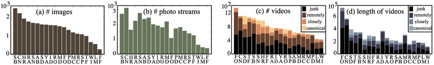
timestamp tli . The likelihood f (P) is defined as follows.                        can reduce the inference of At to a neighborhood selection-
           L
                                                                                   style optimization [14], which enables to estimate the graph
                                                                                   by independently solving a set of atomic weighted lasso
           Y                            Y
  f (P)=     f (P l ), where f (P l ) =   f (xli , tli |xlp(i) , tlp(i) ) (2)
           l=1                               xli ∈P l                              problem for each dimension d while guaranteeing asymp-
where    xlp(i)
             and denote the parent of xli in the directed tree                     totic consistency. Hence, the optimization becomes trivially
                                                                                   parallelizable per dimension. Such property is of particular
T l . Since no vee structure is allowed, each image has only                       importance in our problem possibly using millions of im-
one parent. For the transition model f (xli , tli |xlp(i) , tlp(i) ),              ages with many different image descriptors. Finally, we en-
we use the linear dynamics model, as one of the simplest                           courage a sparse solution by penalizing nonzero elements
transition models for dynamic Bayesian networks (DBN):                             of At . As a result, we estimate At by iteratively solving
             xli = Ae xlp(i) + , where  ∼ N (0, σ 2 I)                     (3)   the following optimization D times:
                                                                                                    L X
                                                                                                    X
where  is a vector of Gaussian noise with zero mean and                           b td∗ = argmin
                                                                                   A                   wt (i)(xli,d − gi Atd∗ xlp(i) )2 + λkAtd∗ k (5)
variance σ 2 . In order to model time difference between                                            l=1 i∈P l

tlp(i) and tli , we use the exponential rate function that is                      where wt (i) is the weighting of an observation of image
widely used for the temporal dynamics of diffusion net-                            pli in photo stream l at time t. That is, if the timestamp
works [17]: the (x, y) element axy of Ae has the form of                           tli of pli is close to t, wt (i) is large so that the observa-
αxy exp(−αxy ∆i ) where ∆i = |tli − tlp(i) | and αxy is the                        tion contributes more on the graph estimation at t. Nat-
transmission rate from visual cluster x to y. As αxy → 0,                                                                    κ (t−tl )
                                                                                   urally, we can define wt (i) = PL Ph κi (t−tl ) where
the consecutive occurrence from x to y is very unlikely. By                                                               l=1   i∈P l   h   i

letting A = {αxy exp(−αxy )}D×D , we have Ae = gi A                                κh (u) is Gaussian RBF kernel√with a kernel bandwidth h
with gi = exp(∆i ).                                                                (i.e. κh (u) = exp(−u2 /2h2 )/ 2πh).
    For better scalability, we impose a practically reasonable                         In Eq.(5), we include `1 -regularization where λ is a pa-
                                                                                   rameter that controls the sparsity of Ab t . It not only avoids
assumption on the transition model. Each visual cluster of                                                                  d∗
xli is conditionally independent of another given xlp(i) . That                    overfitting but also is practical because only a small number
is, the transition likelihood factors                                              of strong story branches at each node are detected so that
                                        QD over individual dimen-                  story links are not unnecessarily complex. Consequently,
sions: f (xli , tli |xlp(i) , tlp(i) ) = d=1 f (xli,d , tli |xlp(i) , tlp(i) ).
Consequently, from Eq.(3), we can express the transition                           our graph inference reduces to iteratively solving a standard
likelihood as Gaussian distribution: f (xli,d , tli |xlp(i) , tlp(i) )             weighted `1 -regularized least square problem, whose global
                                                                                   optimum can be solved by scalable techniques such as the
= N (xli,d ; gi Ad∗ xlp(i) , σ 2 ), where Ad∗ denotes the d-th
                                                                                   coordinate descent [6]. In summary, the graph inference can
row of the matrix A. Finally, the log-likelihood log f (P)
                                                                                   be performed in a linear time with respect to all parame-
in Eq.(2) can be written
                                                                                   ters, including the number of images and nodes. We present
                        L X X
                        X   D                                                      more details of the algorithm including the pseudocode in
    log f (P) = −                       f (xli,d )      where                (4)   the supplementary material.
                        l=1 i∈P l d=1
                                                                                       After solving the optimization of Eq.(5) to discover the
                      Nl

                                       1                                           topology of the storyline graph (i.e. nonzero elements of
   f (xli,d ) =          log(2πσ 2 ) + 2 (xli,d − gi Ad∗ xlp(i) )2
                      2               2σ                                           {At }), we run the parameter learning (i.e. estimating actual
                                                                                   associated weights) while fixing the topology of the graph.
4.3. Optimization                                                                  Since the structure of each graph is known and all photo
                                                                                   streams are independent of one another, we can easily solve
    Our optimization problem is to discover nonzero ele-                           for MLE of A   b t , which is similar to that of the transition
ments of At for any t ∈ [0, T ], by maximizing the log-                            matrix of k-th Markovian chains.
likelihood of Eq.(4). For statistical tractability and scalabil-
ity, we take advantage of the constraints and the assumption                       5. Experiments
described in previous section.
    First, one difficulty during optimization is that for a fixed                     We evaluate the proposed approach from two technical
t, the estimator may suffer from high variance due to the                          perspectives: video summarization in section 5.1 and image
scarcity of training data (i.e. images occurring at time t may                     summarization as storylines in section 5.2.
be too few). In order to overcome this, we take advantage                             Flickr/YouTube dataset. Fig.3.(a)–(b) summarize our
of the constraint that At varies smoothly over time; thus,                         Flickr dataset of 20 outdoor recreational activity classes that
we can estimate At by re-weighting the observation data                            consists of about 2.7M images from 35K photo streams.
near t accordingly. Second, thanks to the conditional inde-                        Some classes are re-used from the datasets of [9], and
pendence assumption per dimension of visual clusters, we                           the others are newly downloaded using the same crawling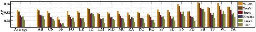
AB (air+ballooning), CN (chinese+new+year), FF (fly+fishing), FO (formula+one), HR (horse+riding), ID (independence+day), LM (london+marathon), MC (moun-
tain+camping), MD (memorial+day), PD (st+patrick+day), RA (rafting), RC (rock+climbing), RO (rowing), SB (surfing+beach), SD (scuba+diving), SN (snowboarding),
SP (safari+park), TF (tour+de+france), WI (wimbledon), YA (yacht).
Figure 3. The Flickr/YouTube datasets of 20 outdoor recreational classes. (a)–(b) The number of images and photo streams of Flickr
dataset: (2,769,504, 35,545). (c)–(d) The number and total length of YouTube videos: (15,912, 1,586.8 hours).
method, in which the topic names are used as search key- Results. Fig.4 reports the average precisions of our al-
words and all queried photo streams of more than 30 images gorithms and baselines across the 20 classes. Our algo-
are downloaded without any filtering. rithm significantly outperforms all the baselines in most
Fig.3.(c)–(d) show the statistics of our YouTube datasets classes. For example, the mean AP of the (OursIV) is
with about 16K user videos. We query the same topic 0.8315, which is notably higher than 0.8046 of the best
keywords using YouTube built-in search engines, and baseline (Spect). The performance of the (KMean) and
download only the Creative Commons licensed videos. the (Spect) highly depends on the number of clusters ν.
Since YouTube user videos are extremely noisy, we man- We change ν from 5 to 25, and report the best results.
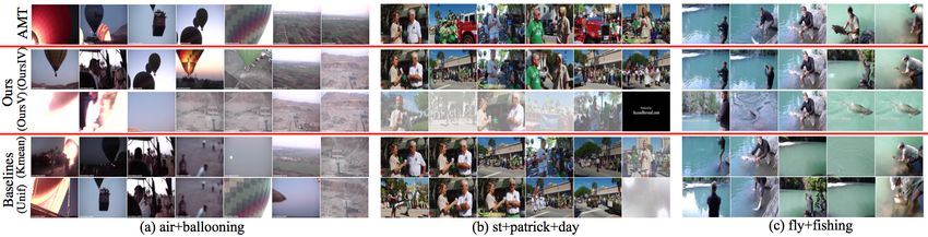
ually rate them into one of four categories: canonical, Fig.5 compares video summarization results produced
closely/remotely related, and junk. These labels are not used by different methods. The (Unif) cannot correctly handle
by the algorithms but for the groundtruth labeling only. different lengths of subshots in a single video (i.e. redun-
dant images can be selected from long subshots while none
5.1. Results on Video Summarization from interesting short ones). One practical drawback of the
(KMean) and the (Spect) is that it is hard to know the best
Tasks. Due to the large-scale nature of our problems,
ν beforehand even though the accuracies highly depend on
we obtain groundtruth (GT) labels via crowdsourcing using
ν. Overall, all algorithms except the (OursIV) suffer from
Amazon Mechanical Turk (AMT), inspired by [8]. For each
the limitations of using low-level features only. For exam-
class, we randomly sample 100 test videos that are rated
ple, as shown in Fig.5.(a), the (OursV) and the (KMean)
as canonical or closely-related, in order to use reasonably
detect meaningless completely-gray sky frames in 3rd and
good videos rather than junk ones for algorithm evaluation.
5th column, respectively. Such frames with no semantic
Then, we uniformly sample 50 frames from each test video,
meaning occur frequently in user videos, whereas very few
and ask at least five different turkers to select 5∼10 ones
in the image sets. Therefore, although (OursIV) uses the
that must be included when they make a storyline summary.
same low-level features, it can easily suppress such unim-
We run our algorithm and baselines to select a small num-
portant information thanks to the similarity votes by the im-
ber of keyframes as a summary of each test video. We then
ages that photographers take more carefully with sufficient
compute the similarity-based average precision (AP) values
semantic intents and values2 .
proposed in [8], by comparing the result to the five GT sum-
maries and then taking the mean of the APs. Finally, we 5.2. Results on Photo Storyline Summarization
compute the mean APs from all annotated test videos. We
defer the detail of the AP computation to the supplementary. Task. It is inherently difficult to quantitatively evaluate
the storyline reconstruction because there is no groundtruth
Baselines. We select four baselines based on the recent available. Moreover, it is painfully overwhelming for a
video summarization studies [8, 12, 13]. The (Unif) uni- human labeler to evaluate the storylines summarized from
formly samples ν keyframes from each test video. The large sets of images. For example, given multiple story-
(KMean) and the (Spect) are the two popular cluster- line graphs with hundreds of nodes created from millions
ing methods, K-means and spectral clustering, respectively. of images, a human labeler may feel hopelessly devastated
They first create ν clusters and select the images closest to to judge which one is better. In order to overcome such in-
the cluster centers. The (RankT) is one of state-of-the-art herent difficulty of the storyline evaluation, we design the
keyframe extraction methods using the rank-tracing tech- following evaluation task via crowdsourcing.
nique [1]. Our video summarization is performed in two
We first run our methods and baselines to generate story-
different ways. The (OursV) denotes our method without
line graphs from the dataset of each class. We then sample
involving similarity votes by images, while the (OursIV) is
our fully-geared method; this comparison justifies the use- 2 Unfortunately, such semantic significance is not fully evaluated by the
fulness of joint summarization between images and videos. AP metric of Fig.4, which is solely based on low-level feature differences.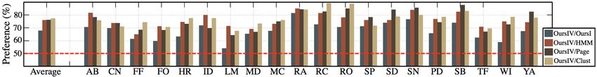
Figure 4. Comparison of mean average precisions (APs) between our methods (OursIV) and (OursV) and the baselines (Unif), (KMean),
(Spect), and (RankT). The acronyms of activities are referred to Fig.3. The leftmost bar set shows the average APs for all classes.
(OursIV): 0.8315, (OursV): 0.8234, (Spect): 0.8046, (KMean): 0.7983, (RankT): 0.7997, and (Unif): 0.7837.

Figure 5. Qualitative comparison of video summarization results. From top to bottom, we show AMT groundtruth and the same number of
selected keyframes by our algorithms (with and without similarity voting by images), and two baselines (KMean) and (Unif).

100 canonical images on the timeline as test instances IQ .         compare with our algorithm using images only, denoted by
Based on the storyline, each algorithm can retrieve one im-         (OursI), in order to quantify the improvement by joint
age that is most likely to come next after each test image          summarization with videos. We present more details of ap-
Iq ∈ IQ . That is, we first identify which node corresponds         plication of our algorithm and baselines in supplementary.
to the Iq , and follow the most strongly connected edge to the          Results. Fig.6 shows the results of pairwise preference
next likely node, from which the central image is retrieved.        tests obtained via AMT between our algorithm and each
For evaluation, a turker is shown the test image Iq , and then      baseline. The number indicates the mean percentage of re-
a pair of images predicted by our algorithm and one of base-        sponses that choose our prediction as a more likely one to
lines in a random order, and asked to choose the one that is        come next after each Iq than that of the baseline. That is,
more likely to follow Iq than the other. We design the AMT          the number should be higher than at least 50% to validate
task as a pairwise comparison instead of a multiple-choice          the superiority of our algorithm. Even considering a certain
question (i.e. selecting the best one among the outputs of all      degree of unavoidable noisiness of AMT labels, our output
algorithms), to make the annotation simple enough for any           is significantly preferred by AMT annotators. For exam-
turker to instantaneously complete. We obtain such pair-            ple, our algorithm (OursVI) gains 75.9% of votes, far out-
wise comparison for each of IQ from at least three different        distancing the best baseline (HMM). Importantly, more than
turkers. In summary, the underlying idea of our evaluation          two thirds of responses (i.e. 67.9%) prefer the results of the
is that we recruit a crowd of labelers, each of who evaluates       (OursVI) over those of the (OursI), which indeed sup-
only a basic unit (i.e. an important edge of the storyline),        port our argument that a crowd of videos help improve the
instead of the assessment of the whole storyline, which is          quality of the storylines from users’ point of view.
practically impossible.                                                 Fig.7 illustrates another interesting qualitative compar-
   Baselines. We compare three baselines with our ap-               ison between our method and baselines. Given a pair of
proach. The (Page) is a Page-Rank based image retrieval             images that are distant in a novel photo stream (i.e. im-
that simply selects the top-ranked image around the times-          ages within red boundaries in Fig.7.(a)), each algorithm pre-
tamp of Iq . It is compared to show that storylines as se-          dicts 10 images that are likely to occur between them using
quential summary can be more useful than the traditional            its own storyline graph (i.e. each algorithm finds out the
retrieval method. The (HMM) is an HMM based method that             best path between the two images). As shown in Fig.7.(a),
has been popularly applied for sequence modeling. This              our algorithm (in the second row) can retrieve the images
comparison can tell the importance of our branching struc-          that are very similar to the hidden groundtruths (in the first
ture over the linear storyline of the (HMM). The (Clust) is a       row). Using the iterative Viterbi algorithm, the (HMM) re-
simple clustering-based summarization on the timeline [9],          trieves reasonably good but highly redundant images, which
in which images are distributed on the timeline of 24 hours,        are in part due to its inability to represent various branch-
and grouped into 10 clusters at every 30 minutes. We also           ing structures. The (Page) retrieves top-ranked images (i.e.
Figure 6. The results of pairwise preference tests between our method (OursIV) and each baseline via Amazon Mechanical Turk. The
numbers indicates the percentage of responses that our prediction is more likely to occur next after Iq than that of the baseline. At least the
number should be higher than 50% (shown in red dotted line) to validate the superiority of our algorithm. The leftmost bar set shows the
average preference of our (OursIV) for all 20 classes: [67.9, 75.9, 76.1, 77.1] over (OursV), (HMM), (Page), and (Clust).

Figure 7. Examples of an qualitative comparison between our method and baselines. (a) Given a pair of distant images in a photo stream
(i.e. the ones within red boundaries), each algorithm predicts the best path between them and samples 10 images. (b) A downsized version
of our storyline graph used for the prediction of (a).

representative and high-quality images) at each query time                 [7] A. Gupta, P. Srinivasan, J. Shi, and L. S. Davis. Understanding
point. However, it has no use of the sequential structure, and                 Videos, Constructing Plots: Learning a Visually Grounded Storyline
                                                                               Model from Annotated Videos. In ICCV, 2009. 2
thus there is no connected story between retrieved images.                 [8] A. Khosla, R. Hamid, C. J. Lin, and N. Sundaresan. Large-Scale
Fig.7.(b) shows a downsized version of our storyline graph                     Video Summarization Using Web-Image Priors. In CVPR, 2013. 2,
that is used for creating the result of Fig.7.(a). Although we                 3, 6
can freely choose the temporal granularity to zoom in or out               [9] G. Kim and E. P. Xing. Jointly Aligning and Segmenting Multiple
                                                                               Web Photo Streams for the Inference of Collective Photo Storylines.
the storylines, we here show only a small part of them for                     In CVPR, 2013. 2, 5, 7
better visibility. We present more illustration examples of               [10] G. Kim, E. P. Xing, L. Fei-Fei, and T. Kanade. Distributed Coseg-
storyline graphs in the supplementary.                                         mentation via Submodular Optimization on Anisotropic Diffusion.
                                                                               In ICCV, 2011. 3, 4
6. Conclusion                                                             [11] M. Kolar, L. Song, A. Ahmed, and E. P. Xing. Estimating Time-
                                                                               Varying Networks. Ann. Appl. Stat., 4(1):94–123, 2010. 4
   In this paper, we proposed a scalable approach to jointly              [12] Y. J. Lee, J. Ghosh, and K. Grauman. Discovering Important People
summarize large sets of Flickr images and YouTube videos,                      and Objects for Egocentric Video Summarization. In CVPR, 2012.
                                                                               2, 6
and created a novel structural summary as storyline graphs                [13] Z. Lu and K. Grauman. Story-Driven Summarization for Egocentric
visualizing a variety of underlying narrative branches of                      Video. In CVPR, 2013. 2, 6
topics. We validated the superior performance of our ap-                  [14] N. Meinshausen and P. Bühlmann. High-Dimensional Graphs and
proach via the evaluation using Amazon Mechanical Turk.                        Variable Selection with the Lasso. Ann. Statist., 34(3):1436–1462,
                                                                               2006. 5
                                                                          [15] H. Misra, F. Hopfgartner, A. Goyal, P. Punitha, and J. M. Jose. TV
References                                                                     News Story Segmentation Based on Semantic Coherence and Con-
 [1] W. Abd-Almageed. Online, Simultaneous Shot Boundary Detection             tent Similarity. In MMM, 2010. 2
     and Key Frame Extraction for Sports Videos Using Rank Tracing. In    [16] A. Prest, C. Leistner, J. Civera, C. Schmid, and V. Ferrari. Learning
     ICIP, 2008. 6                                                             Object Class Detectors from Weakly Annotated Video. In CVPR,
 [2] O. Boiman, E. Shechtman, and M. Irani. In Defense of Nearest-             2012. 2
     Neighbor Based Image Classification. In CVPR, 2008. 3                [17] M. G. Rodriguez, D. Balduzzi, and B. Schölkopf. Uncovering the
 [3] C. Y. Chen and K. Grauman. Watching Unlabeled Video Helps Learn           Temporal Dynamics of Diffusion Networks. In ICML, 2011. 5
     New Human Actions from Very Few Labeled Snapshots. In CVPR,          [18] I. Simon, N. Snavely, and S. M. Seitz. Scene Summarization for
     2013. 2                                                                   Online Image Collections. In ICCV, 2007. 2
 [4] L. Chen, L. Duan, and D. Xu. Event Recognition in Videos by Learn-   [19] L. Song, M. Kolar, and E. Xing. Time-Varying Dynamic Bayesian
     ing from Heterogeneous Web Sources. In CVPR, 2013. 2                      Networks. In NIPS, 2009. 4
                                                                          [20] K. Tang, V. Ramanathan, L. Fei-Fei, and D. Koller. Shifting Weights:
 [5] J. Deng, W. Dong, R. Socher, L. J. Li, K. Li, and L. Fei-Fei. Ima-
                                                                               Adapting Object Detectors from Image to Video. In NIPS, 2012. 2
     geNet: A Large-Scale Hierarchical Image Database. In CVPR, 2009.
                                                                          [21] A. Torralba, R. Fergus, and W. T. Freeman. 80 Million Tiny Images:
     2
                                                                               A Large Data Set for Nonparametric Object and Scene Recognition.
 [6] W. J. Fu. Penalized Regressions: The Bridge Versus the Lasso. J.
                                                                               IEEE PAMI, 30:1958–1970, 2008. 2, 3
     Computational Graphical Statistics, 7:397–416, 1998. 5
You can also read