Vostok: 3D scanner simulation for industrial robot environments - ddd-UAB
←
→
Page content transcription
If your browser does not render page correctly, please read the page content below
Electronic Letters on Computer Vision and Image Analysis 19(3):71-86, 2020

Vostok: 3D scanner simulation for industrial robot environments

                            Alessandro Rossi†∗ , Marco Barbiero∗ and Ruggero Carli∗

                                                †
                                                 Euclid Labs s.r.l., Treviso, Italy
                            ∗
                                Department of Information Engineering, University of Padova, Italy

                                  Received 1st of June 2020; accepted 19th of September 2020

                                                          Abstract
          Computer vision will drive the next wave of robot applications. Latest three-dimensional scanners pro-
      vide increasingly realistic object reconstructions. We introduce an innovative simulator that allows inter-
      acting with those scanners within the operating environment, thus creating a powerful tool for developers,
      researchers and students. In particular, we present a novel approach for simulating structured-light and time-
      of-flight sensors. Qualitative results demonstrate the efficiency and reliability in industrial environments. By
      using the programmability of modern GPUs, it is now possible to make greater use of parallelized simulative
      approaches. Apart from the easy modification of sensor parameters, the main advantage in simulation is the
      opportunity of carrying out experiments under reproducible conditions, especially for dynamic scene setups.
      Moreover, thanks to a great computational power, it is possible to generate huge amounts of synthetic data
      which can be used as test datasets for training machine learning models.

      Key Words: Structured-Light, Time-of-Flight, Ray Tracing, Computer Vision, Robotics, Synthetic Data

1    Introduction
Due to recent technology improvements, we are now getting close to a next era of robots in which they will do
multiple tasks, and computer vision will play a huge role in that. It allows robots to see what is around them
and make decisions based on what they perceive. Through new technologies, such as deep learning, robots
can interpret these images and learn new things on the fly. The industrial automation demands faster machine
cycles, shorter installation times and greater customization. To meet these requirements, new tools are needed to
analyse the project in advance, highlighting peculiarities and complexities. To address this requirement, Euclid
Labs, an innovative company in machine vision field and, in particular, over bin picking solutions, presents
Vostok: a powerful simulator, that will be a state-of-the-art tool for developers, researchers and students [1].
This software allows to design a real workcell adding robots, vision and I/O systems, sensors, conveyor belts,
and more. An example of a simulated workcell is shown in Figure 1. Then the user can program robots, test
their behaviours, grab photos or trigger scanners to generate point clouds. The user could also connect the
    Correspondence to: ale.rossi.mn@gmail.com
    Recommended for acceptance by Angel D. Sappa
    https://doi.org/10.5565/rev/elcvia.1244
    ELCVIA ISSN: 1577-5097
    Published by Computer Vision Center / Universitat Autònoma de Barcelona, Barcelona, Spain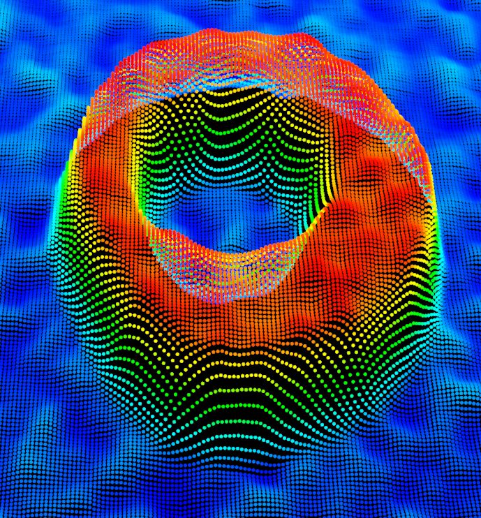
72             A. Rossi et al. / Electronic Letters on Computer Vision and Image Analysis 19(3):71-86, 2020

entire workcell to a proprietary system, allowing to test very complex algorithms without having real expensive
robots or scanners.

                                     Figure 1: A Vostok workcell example.

    In this paper, we present only some features of this software and, in particular, we focus on 3D scanners sim-
ulation. Actually, surface reconstruction constitutes a fundamental topic in computer vision, having different
applications such as object recognition and classification, pick and place, and industrial inspection. Developed
solutions are traditionally categorized into contact and non-contact techniques [2]. The former were used for
a long time in industrial inspections and consist of a tool which probes the object through physical touch. The
main problems of contact techniques are their slow performance and high cost of using mechanically calibrated
passive arms. Besides, the fact of touching the object is not feasible for many applications. Non-contact tech-
niques were developed to cope with these problems and have been widely studied. They can be classified into
two different categories: active and passive. The former exploits reflectance of the object and scene illumina-
tion to derive shape information: no active device is necessary [3]. An example is stereo-vision, where scene is
first imaged by cameras from two or more points of view and then correspondences between images are found.
The main problem experimented using this approach is sparse reconstruction since density is directly related to
object texture. This complicates the process of finding correspondences in presence of texture-less surfaces. On
the other hand, in active approaches, suitable light sources are used as internal vector of information. Among
those, two of the most popular methods are definitely structured-light and time-of-flight reconstructions. Within
this work we propose a novel approach to simulate these scanners. Our aim was to create a useful simulator for
the design of automated cells. In this field the acquisition time of a 3D image is very low. To correctly estimate
the cycle time, the simulation must provide a reliable result in the shortest time possible and should not take
longer than a real scanner. In the literature we find very complex models whose aim is to achieve the maximum
realism without worrying about the actual applicability in the industrial field. For this reason, it was necessary
to find a trade-off between simulation speed and accuracy. For example, the methods provided by Zanuttigh et
al. allow to simulate most of the effects of rays’ light reflection and refraction but they are too complex from a
computational point of view to be used for our purpose [4]. So, we decided to use a one-hop ray tracing model
in which only the first reflection of light is traced. This model allowed to drastically reduce the computation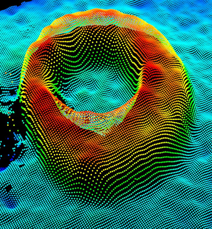
A. Rossi et al. / Electronic Letters on Computer Vision and Image Analysis 19(3):71-86, 2020           73

time and, at the same time, to preserve a good accuracy in standard situations, as shown in Section 4.
   This paper is organized as follows. Section 2 shows the problem formulation in detail. Section 3 presents
design and software implementation of the simulator. Special emphasis is placed on its limits, highlighting
possible future improvements too. In Section 4 algorithms are tested with different types of objects analysing
quality, precision and deviation from the results given by real scanners. We highlight how GPU computing
helped to dramatically reduce computational time. Finally, concluding remarks and possible extensions are
presented in Section 5.

2     Theoretical models
In this section we provide basic operating principles of the two simulated sensors to highlight the foundations
on which the simulator is based.

2.1    Structured-light technique
This reconstruction technique consists in retrieving the three-dimensional surface of an object by exploiting
the information derived from the distortion of a projected pattern. Differently from stereo vision approach,
one of the cameras is substituted by an active device which projects a structured-light pattern onto the scene.
This active device can be modelled as an inverse camera, being the calibration step a similar procedure to
the one used in classical stereo vision systems. An imaging sensor is used to acquire an image of the scene
under structured-light illumination. If the scene consists of a planar surface, the pattern in the acquired image
would be similar to the projected one. However, when the surface is non-planar, its geometric shape distorts the
projected pattern as seen from the camera. The principle of structured-light imaging techniques is to derive the
missing depth information from the distortion of the projected pattern. Accurate 3D surface profiles of objects
in the scene can be computed by using various structured-light approaches and algorithms [5].

                                 Prj                                            Cam

                                                         b

                                                α                  β

                                                                    d

                                                    P1

                                          P2

                           Figure 2: Operation principle of a structured-light scanner.

    As shown in Figure 2, the geometric relationship between an imaging sensor, a structured-light projector and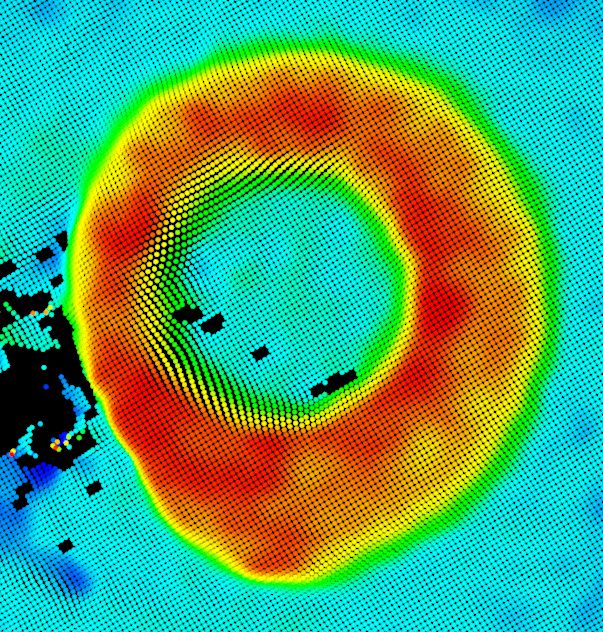
74             A. Rossi et al. / Electronic Letters on Computer Vision and Image Analysis 19(3):71-86, 2020

a surface point, can be expressed by the triangulation principle as
                                                          sin α
                                                d=b                                                           (1)
                                                       sin(α + β)
From the figure we can immediately observe the main limitation of this technique: the presence of occlusions.
In fact, these can be generated in two cases. The first case occurs when the pattern does not cover the entire
surface because some parts generate shadows. The other case occurs when a projected point cannot be identified
from the camera’s point of view (represented by point P2 in the example in Figure 2).
   Over the past years, structured-light projection systems have been widely studied. Since the 70’s, several
researchers have proposed different solutions to recognise polyhedral and curvilinear objects, as evidenced by
several works [6–9]. The tipping point took place in 1986 when Stockman et al. have proposed the widely
known projection of a grid [10]. Since then, several points could be processed in parallel and an easier corre-
spondence problem has to be solved: we have to identify, for each point of the imaged pattern, the correspond-
ing point of the projected one. The correspondence problem can be directly solved codifying the projected
pattern, so that each light point carries some spatial information. A detailed survey on recent progress in coded
structured-light is presented by [11]. Although many variants of structured-light systems are possible, binary
codes are widely used. They basically consist in parallel stripes patterns and an example is given in Figure 3.

                             Figure 3: Sequential binary-coded pattern projections.

   Depending on the camera resolution, such a system allows digitizing several hundred thousand points at
a time. The main advantage of this technology regards precision: distance resolution is about 1 mm. In
addition, these scanners can be used in dark environments and they are not sensible to brightness changes. The
main drawback is represented by physical characteristics of the material: for instance, specular surfaces causes
significant errors during depth reconstruction. Moreover, we already encountered the issue of occlusions which
gets worse with the increase in the baseline, that is the distance between camera and projector.

2.2   Time-of-flight technique
This technique retrieves depth information by estimating the elapsed time between the emission and receipt
of active light signals. Several different technologies for those cameras have been developed but the most
common are continuous-wave and pulsed light [12]. In the latter, a camera illuminates the scene with modulated
incoherent near-infrared light. The illumination is switched on for a very short time. The resulting light pulse
illuminates the scene and is reflected by the objects in the field of view. The camera lens gathers the reflected
light and images it on the sensor. An optical band-pass filter only passes the light with the same wavelength as
the illumination unit, to reduce background light and noise effects. Depending upon the distance, the incoming
light experiences a delay. As speed of light is approximately 3 × 10⁸ m/s, this delay is very short. Each smart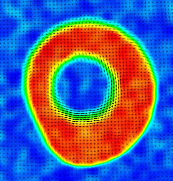
A. Rossi et al. / Electronic Letters on Computer Vision and Image Analysis 19(3):71-86, 2020          75

pixel measures the time the light has taken to travel from the illumination source to the object and back to the
image plane. Thus, the camera can determine the distance to the corresponding object region. The pulse width
of the illumination determines the maximum range the camera can handle. With a pulse width of 40 ns, the
range is limited to
                                     1          1
                            dmax =     · c · t ' · 3 × 10⁸ m/s · 40 × 10−9 s = 6 m                             (2)
                                     2          2

Continuous-wave modulation technique is described in detail by Georgiev et al. with excellent emphasis on
noise modelling [13, 14].

                                                    IR           Cam

                            Figure 4: Operation principle of a time-of-flight camera.

   The distance resolution is about 1 cm and so spatial resolution is generally low compared to structured-light
scanners. However, time-of-flight cameras operate very quickly: they can measure the distances within a scene
in a single shot. In fact, they are ideally suited for real-time applications. Moreover, distance reconstruction
algorithm is very efficient. As a result, the computational power required is much lower than in structured-light
approaches, where complex correlation algorithms are implemented. Finally, the whole system is very compact:
the illumination is placed close to the lens, whereas other systems need a certain minimum baseline. Among
drawbacks we underline the sensibility to background light. Sun and artificial lighting can be stronger than the
modulated signal and this can significantly ruin the reconstruction. In contrast to laser scanning systems where
a single point is illuminated, time-of-flight cameras illuminate the whole scene. Due to multiple reflections,
the light may reach the objects along several paths. Therefore, the measured distance may be greater than the
true one. Besides, since those cameras use active illumination - infrared light - to measure distances, they are
sensible to error from reflections in their surroundings. This phenomenon is accentuated along vertical faces of
objects and causes the presence of detected points that do not belong to the object surface; they are called flying
pixels.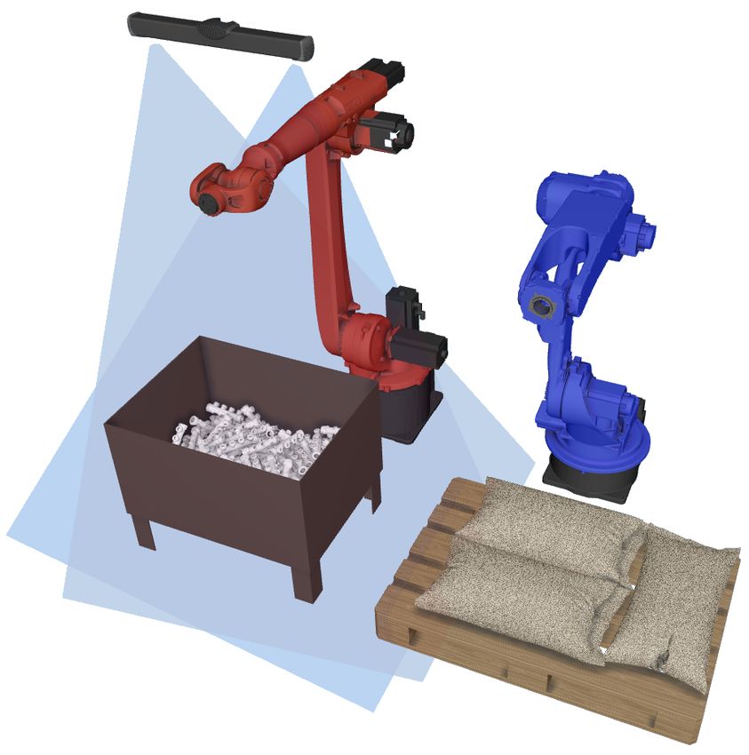
76             A. Rossi et al. / Electronic Letters on Computer Vision and Image Analysis 19(3):71-86, 2020

3     Algorithms and Implementation
Our aim is to replicate the results obtained by these three-dimensional scanners with a good level of realism.
As briefly shown in Section 2, scanners operating principles usually depend on elements that are very tricky to
replicate. A clear example is represented by light which strongly affects the result of a reconstruction. Accu-
rately simulating the behaviour of light is very complex and still subject of research. In addition, introducing
the concept of time, within the simulator, is unnecessary, since precise distances are automatically available by
construction. Therefore, (2) cannot be applied directly in the time domain. Actually, the difficult and interesting
part of building a ToF simulator is to reproduce quantization, saturation and noise effects as they are defined
in the time domain. To overcome this problem, we do all the computations in the space domain by inverting
the formula, since light propagation time is linearly linked to distance by the constant c. The section begins by
describing the implementation choices in simulating the two types of scanners and ends with an emphasis on
the use of GPU computing and some further optimizations.

3.1   Structured-light scanner simulation
We have already observed how this kind of scanners have a very good accuracy in terms of distance resolution.
The main characteristic of these reconstructions is certainly the presence of occlusions. The greater the baseline,
the greater this effect will be. Considering a complex object, characterized by numerous edges, it is very likely
that parts of the projected pattern are not visible from the perspective of the camera, thus causing occlusions. To
reproduce this main feature, it is unnecessary to replicate in detail the theoretical model. One way to proceed
is to simulate the path of light rays. In computer science, the most popular technique is ray tracing [15]. Given
a projection pattern, in our case a grid of points, an iteration of that algorithm is performed for each point.
Given the projector’s origin, a ray is launched through each point of the pattern and its path is traced to the
intersection with the objects in the scene. Since a mesh is a set of triangles, this operation is based on a ray-
triangle intersection method; in particular we have chosen the Möller-Trumbore algorithm which represents the
state-of-the-art for this task and uses minimal system memory [16, 17]. Finally, starting from this intersection,
we search for a trajectory compatible with the camera focal plane. To increase the level of realism, only the
reflected component of the ray, obtained through Snell’s law, given the refractive index of the material, is taken
into account. To be more precise, it would be possible to trace rays’ reflections even after the first intersection,
but this would increase the computational load. However, the advent of a new generation of Nvidia RTX GPUs
will make this process much faster thanks to the hardware implementation of part of the ray tracing procedure.

3.2   Time-of-flight camera simulation
A valid simulation approach is that provided by Keller et al. [18]. They proposed a pixel-wise simulation
approach, exploiting the depth map, an image that contains information relating to the distance of scene objects’
points from a particular viewpoint, automatically available after rendering in GPU. This approach makes the
process very fast, almost real-time, but the limitation to per-pixel data causes inaccuracy in the reconstruction.
In fact, among the drawbacks of a time-of-flight camera, we already observed the presence of the so-called
flying pixels (see Figure 5).
    This effect is difficult to implement using this approach, because no information about the surrounding pixels
exists while processing a single pixel at the GPU. So, as for the structured-light scanner simulation, we decided
to use a ray tracing approach. In particular, we trace the path of IR rays, measuring the time the light has
taken to travel from the illumination source to the object and back to the image plane. We have implemented a
first-hop ray tracing algorithm. We could increase the realism by considering further reflections of light rays.
By using this approach, based on ray tracing, prevents a real-time reconstruction but allows to reproduce the
flying pixels phenomenon because it considers the surroundings of each pixel. Another feature of time-of-flight
reconstructions, which differs from structured-light ones, is the pronounced presence of noise. This is due to a
lower accuracy and to the problem of multiple reflections, which causes the estimated distance to be greater than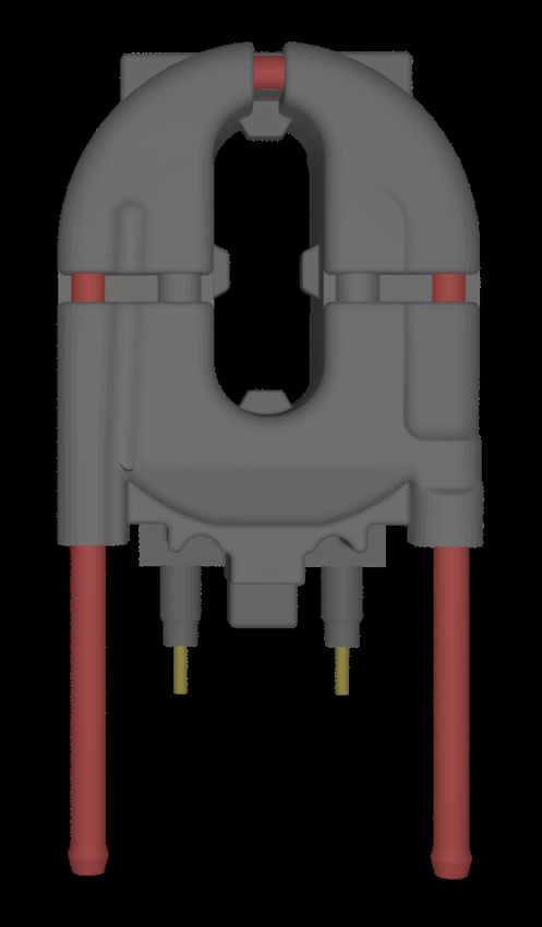
A. Rossi et al. / Electronic Letters on Computer Vision and Image Analysis 19(3):71-86, 2020            77

Figure 5: Simulated reconstruction of the object in Figure 2. The presence of flying pixels is very clear on
vertical faces of the object.

the real one. Moreover, the electronic components of a camera react sensitively to a variation in temperature.
In addition to the thermal noise, the signal is also influenced by dark current and reset noises. Thus, the noise
produced by a time-of-flight sensor is still subject of current research. We decided to approximate the sum
of all these noises with a Gaussian normal distribution. The inspiration comes from the studies [13, 14] that
describe a noise model for low sensing environments. In these, a ToF device works in suboptimal conditions
(e.g. low emitting power) and delivers measurement errors considerably higher than in a standard operating
mode. They also proved that in usual environments, as in our case, it is possible to describe noise through a
Gaussian distribution. Future developments will certainly include improving the noise model in order to make
the reconstruction more faithful.

3.3   GPU computing
As soon as the simulated framework is outlined, the need of massive GPU parallel computing becomes clear.
For instance, a ray tracing algorithm requires the computation of millions, or even billions, of intersections.
Even a top range CPU could never complete such a task in a reasonable time. Therefore, we decided to use
DirectCompute, a DirectX 11 feature, which allows using graphics processing units for general purposes other
than graphic rendering. The greatest benefit of DirectCompute, over other rendering APIs, such as CUDA or
OpenGL, is that algorithm performance can easily scale with the user hardware. We do not focus on this issue
because it would deserve a separate discussion. We just want to reiterate the need of using graphical resources
to implement this kind of algorithms. In this regard, in Section 4 we compare CPU and GPU performance
during simulation. For further information regarding DirectCompute and its use, please refer to the books [19]
and [20].

3.4   Further optimizations
One of the optimizations that deserves a separate discussion regards the use of voxeling [21, 22]. During
an iteration of the ray tracing algorithm, it is necessary to search for all the intersections between a ray and
object surfaces. An elaborate scene will have many objects and consequently lots of triangles. Therefore, the
intersection search becomes a complex computational task. Instead of using a brute-force approach and cycling
across all triangles of the scene, one might think about how to reduce the number of searches. One idea is to
implement a step-by-step search algorithm, exploiting the bounding box of each object. The latter is defined
as the parallelepiped with the smallest volume containing all the points of the object. We also introduce the
concept of voxel as a further subdivision of the bounding box. In our case, a bounding box is divided into 8
voxels. This partitioning can be iterated and, at the second step, we find 64 voxels. In this way we transform
the ray-triangle intersection problem into a ray-box intersection one. First of all, ray-box intersection algorithm
is much simpler and faster than the ray-triangle algorithm provided by Möller-Trumbore, but especially voxels
are incredibly less than triangles. Once we have intersected a particular voxel, we search for the intersections
with the triangles it contains, which are a small part of the total. This has allowed us to significantly reduce
78             A. Rossi et al. / Electronic Letters on Computer Vision and Image Analysis 19(3):71-86, 2020

reconstruction time. The algorithm in pseudo-code is given below, while an useful representation is shown in
Figure 6.

Algorithm 1 Ray-triangle intersection using voxeling
    Input: ray r, list of bounding boxes bList (one for each mesh)
    Output: intersected triangle t
 1: procedure I NTERSECT(r, bList)
 2:    for all b ∈ bList do
 3:        if r intersects b then
 4:             for all v ∈ b.voxels do                      . b.voxels are the 8 voxels of the bounding box b
 5:                 if r intersects v then
 6:                      for all w ∈ v.voxels do                    . v.voxels are the 8 voxels of the voxel v
 7:                          if r intersects w then
 8:                               for all t ∈ w.triangles do
 9:                                   if r intersects t then
10:                                        return t
11: end procedure

                           ray r

                                                                              bounding box b

                                                                             1st depth voxel v

                                                                             2nd depth voxel w

                                    1          1/8   1/64

                     Figure 6: Ray-triangle intersection search using a voxeling approach.

   Simulations showed two main limits to the use of voxeling. First of all, this approach requires a long
initialization. Actually, each triangle must be uniquely associated to a voxel but some may lie on multiple
voxels at once. Therefore, it is necessary to process these triangles separately, making optimization impossible.
The second limit regards the numbers of triangles per bounding box. If these are few, we observed how the
initialization procedure takes more time than using a brute-force approach.

4    Results
In this section we validate the simulator and compare its results with those provided by real scanners. Secondly,
we demonstrate the huge contribution by using GPU computing. To carry out tests we used a workbench
equipped with an Intel Core i7-7700, 16 GB of RAM and an Nvidia GTX 1060. To make comparisons among
A. Rossi et al. / Electronic Letters on Computer Vision and Image Analysis 19(3):71-86, 2020 79
real and simulated results, we used two different structured-light scanners (Zivid One [23] and Photoneo PhoXi
L [24]) and a time-of-flight camera (ODOS StarForm Swift [25]).
Firstly, we want to validate simulator performance. Actually, we are interested in comparing simulated and
real point clouds using concrete industrial samples, in particular those shown in Figure 7. To make this measure,
we used the Iterative Closest Point (ICP) algorithm [26] to minimize the difference between two point clouds.
Briefly, this algorithm keeps one point cloud fixed, while the other one is transformed to maximize the matching
score. To be more precise, we define with S the set of simulated points and with P the set of points belonging
to a real scanner reconstruction. Then, we define the intersection between the two sets as Γ = S ∩ P. At this
point let us define
|Γ| |Γ|
score = , coverage =
|S| |P|
The drawback is that this kind of algorithms also tends to fit noise. Therefore, especially in case of a time-of-
flight reconstruction, this performance index has to be considered qualitatively. However, regarding the results
of structured-light scanners, this index can be taken into account because the amount of noise present is much
lower. Anyway, the images shown are very informative and can therefore be considered an additional index
about the results consistency.
(a) Test sample #1 (b) Test sample #2 (c) Test sample #3 (d) Test sample #4
Figure 7: A view of the industrial samples used for simulation tests.
4.1 Structured-light simulation
For tests we used two different structured light scanners: a Zivid One, with a baseline of 150 mm, and a Pho-
toneo L, with a baseline of 550 mm. Both provide images at a resolution of 1920 × 1080 pixels. The operating
principle is similar but the main difference between the two lies in the type of light projected. In fact, Zivid ex-
ploits a white visible light projection system while Photoneo uses a coherent laser radiation projection system.
This leads to slightly different results but, for our simulation purposes, the main parameter is baseline. Given the
larger baseline of Photoneo L, compared to Zivid One, we can easily imagine that the former is more suitable
for capturing larger scenes. Figure 8 shows a comparison between simulated and real reconstructions obtained
using both scanners. We then overlapped point clouds using the fitting algorithm described at the beginning
of this section. We immediately notice how results, in general, are excellent. In particular, by comparing sim-
ulated and Zivid reconstructions for the test sample #1, the fitting algorithm gives us a score of 94.64% and
a coverage of 99.33%. Table 1 shows the results obtained with various test samples presented in Figure 7.
Actually, as expected, the choice to implement a 1-hop ray tracing algorithm leads to simplify a bit the model.
On the contrary, by using multiple-hop ray tracing, we could replicate the reflection phenomenon. Instead, by
comparing simulated and Photoneo reconstructions, we can observe slightly more differences. Indeed, score
(89.52%) and coverage (90.96%) values drop a bit. The reason for the lower likelihood can be addressed to
the larger baseline and to the particular laser-based projection system used by Photoneo. The latter emphasizes80 A. Rossi et al. / Electronic Letters on Computer Vision and Image Analysis 19(3):71-86, 2020
reflection phenomena and, indeed, we can notice a lower fidelity in the most complex parts of the object (on the
right side and within the interior parts on top). Once again, by increasing the maximum number of reflections in
the ray tracing algorithm, we could improve the result at the cost of a slower simulation. Anyway, by observing
the figures, it is clear how the simulator can be a valid tool to evaluate occlusion and shadow phenomena. For
instance, we can change the baseline or the working distance and see the effect immediately.
(a) Original Zivid (b) Simulated Zivid
(c) Original Photoneo (d) Simulated Photoneo
Figure 8: Structured-light simulated point clouds (in blue) compared with real reconstructions (in red).A. Rossi et al. / Electronic Letters on Computer Vision and Image Analysis 19(3):71-86, 2020 81
Table 1: Results of the comparison between simulated and real point clouds. Real 3D scans were obtained by
using two different scanners: a Zivid One [23] (baseline: 150 mm, working distance: 600 mm) and a Photoneo
PhoXi L [24] (baseline: 550 mm, working distance: 1000 mm).
Model Baseline [mm] Working Distance [mm] Coverage Score
Test sample #1 150 600 99.33 % 94.64 %
Test sample #2 150 600 89.83 % 94.46 %
Test sample #3 150 600 97.09 % 99.94 %
Test sample #1 550 1000 90.96 % 89.52 %
Test sample #2 550 1000 73.86 % 69.54 %
Test sample #3 550 1000 96.73 % 99.86 %
4.2 Time-of-flight simulation
As already observed in Section 3, time-of-flight reconstructions are characterized by a lower accuracy (±1 cm)
and a larger noise component. Despite this, we were able to characterise the noise distribution well. In the
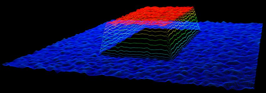
example shown in Figure 9, the object - a motor cam - was scanned at a working distance of 80 cm using the
ODOS camera with an image resolution of 640 × 480 pixels. The same specifications were used within the
simulator to have a common starting point. We can observe that simulation results resemble closely the real
ones of a ToF sensor. We immediately notice the lack of some points in the real image on the right. The reason
is due to the particular reflection of IR rays. The camera used for the experiment has a pulse width of 40 ns.
Therefore, if the elapsed time between the emission and receipt of the light signal take more than 40 ns, then it is
no more considered. Secondly, it may happen that some rays are reflected outside the image plane of the camera
and, then, do not carry information. Finally, a further cause can be found in the pronounced noise that would
have been generated in that area. Despite this, the overall result is promising, as the main point cloud features
have been simulated correctly. By comparing Figures 9c and 9d, we observe how noise modelling also seems
to produce consistent results. In this case, we are not able to provide quantitative results as done previously for
structured light scanners simulation. Actually, the fitting algorithm used to estimate score and coverage between
simulated and real point clouds would also try to fit the noise, thus returning totally meaningless numbers.
4.3 GPU vs CPU
Initially, the simulator was developed entirely to be performed on CPU, using parallel threading to exploit all
the available power. However, we immediately realized that, by increasing the number of projected points, the
time required for a reconstruction gradually became too high. Therefore, we decided to rewrite a big portion of
code to take advantage of GPU computing. In order to highlight the improvements achieved through this step,
we compared GPU and CPU reconstruction performances of the structured-light scanning algorithm by means
of a throughput metric. This is the most natural way to compare the two resources, since we are interested to use
the one that maximizes the numbers of rays computed in the same time unit. Figure 10a shows the throughput
of GPU and CPU using six different pattern densities. The maximum throughput (about 3.5 × 10⁵ rays/s) is
reached by using a GPU along with a very dense projection pattern. Indeed, as reported in Figure 10b, this
corresponds to a speed-up factor of about 40. This is due to the fact that a mid-range GPU has about a thousand
cores that work parallelly, while a common CPU only four. Actually, the most interesting part of Figure 10a is
the bottom left-hand side, i.e. what happens by using a non-dense pattern. In this case, GPU initialization takes
most of the time and, therefore, the throughput is not maximized. Anyway, the speed-up is higher than 10 and
then it is recommended to always exploit GPU acceleration, even for low resolution patterns.82 A. Rossi et al. / Electronic Letters on Computer Vision and Image Analysis 19(3):71-86, 2020
(a) Original ODOS (b) Simulated ODOS
(c) Original ODOS (d) Simulated ODOS
Figure 9: Time-of-flight simulated point clouds compared with real reconstructions of test sample #4. The
colour range is used to indicate depths along z-axis.
106 50×
45×
40×
Throughput [rays/s]
35×
GPU Speedup
5
10 30×
GPU
CPU 25×
20×
15×
104 10×
5×
0×
0 0.5 1 1.5 2 2.5 3 3.5 4 ×10⁶ 0 0.5 1 1.5 2 2.5 3 3.5 4 ×10⁶
pattern points pattern points
(a) CPU vs. GPU Throughput (b) Speedup Factor
Figure 10: Comparison between GPU and CPU reconstruction performances using a structured-light approach.
Figure (a) shows the throughput, whereas Figure (b) shows the speed-up factor gained using GPU instead of
CPU.A. Rossi et al. / Electronic Letters on Computer Vision and Image Analysis 19(3):71-86, 2020 83
5 Conclusions
Along this paper we presented only one of the many facets of Vostok simulator. Specifically, we focused on
the emulation of two 3D reconstruction techniques: structured-light and time-of-flight. Results showed the
simulator offers a good level of realism. Both qualitatively and quantitatively it is quite difficult to distinguish
among real and simulated point clouds. Certainly, as already observed in previous sections, the models can
be expanded and improved. A first idea concerns a more faithful implementation of ray tracing, by tracing
the rays path even after the first reflection. A second point regards noise modelling, which we have seen
heavily corrupting time-of-flight reconstructions. Regardless, simulator performances are sufficient to test any
computer vision algorithm without having real expensive 3D scanners. Furthermore, we will add the possibility
to emulate other reconstruction techniques, e.g. stereo vision. Vostok allows also to simulate 2D cameras,
including lens distortion effects, but this chapter deserves a separate discussion, maybe subject of a future
paper. In conclusion, there are many possibilities offered by the proposed simulator. Computer vision will
drive the next wave of robot applications and deep learning plays a huge role in that. One of the main problems
regards the availability of data to train those systems. With this aim in mind, Vostok would be a powerful tool
to generate test datasets in negligible time.
References
[1] “Vostok 3D Studio,” https://www.vostok3dstudio.com/.
[2] J. Salvi, S. Fernandez, T. Pribanic, and X. Llado, “A state of the art in structured light patterns for surface
profilometry,” Pattern Recognition, vol. 43, no. 8, pp. 2666 – 2680, 2010.
[3] G. Sansoni, M. Trebeschi, and F. Docchio, “State-of-the-art and applications of 3d imaging sensors in
industry, cultural heritage, medicine, and criminal investigation,” Sensors, vol. 9, no. 1, pp. 568–601,
2009.
[4] P. Zanuttigh, L. Minto, G. Marin, F. Dominio, and G. Cortelazzo, Time-of-flight and structured light depth
cameras: Technology and applications. Springer International Publishing, 01 2016.
[5] J. Geng, “Structured-light 3d surface imaging: a tutorial,” Adv. Opt. Photon., vol. 3, no. 2, pp. 128–160,
Jun 2011. [Online]. Available: http://aop.osa.org/abstract.cfm?URI=aop-3-2-128
[6] Y. Shirai, “Recognition of polyhedrons with a range finder,” Pattern Recognition, vol. 4, no. 3, pp. 243–
250, 1972.
[7] G. J. Agin and T. O. Binford, “Computer description of curved objects,” in Proceedings of the 3rd in-
ternational joint conference on Artificial intelligence. Morgan Kaufmann Publishers Inc., 1973, pp.
629–640.
[8] R. J. Popplestone, C. M. Brown, A. P. Ambler, and G. Crawford, “Forming models of plane-and-cylinder
faceled bodies from light stripes.” in IJCAI, 1975, pp. 664–668.
[9] M. Asada, H. Ichikawa, and S. Tsuji, “Determining surface orientation by projecting a stripe pattern,”
IEEE Transactions on Pattern Analysis and Machine Intelligence, vol. 10, no. 5, pp. 749–754, 1988.
[10] G. Stockman and G. Hu, “Sensing 3-d surface patches using a projected grid,” in Computer Vision and
Pattern Recognition, 1986, pp. 602–607.
[11] J. Batlle, E. Mouaddib, and J. Salvi, “Recent progress in coded structured light as a technique to solve the
correspondence problem: a survey,” Pattern recognition, vol. 31, no. 7, pp. 963–982, 1998.84 A. Rossi et al. / Electronic Letters on Computer Vision and Image Analysis 19(3):71-86, 2020
[12] X. Luan, “Experimental investigation of photonic mixer device and development of tof 3d ranging systems
based on pmd technology /,” 01 2001.
[13] M. Georgiev, R. Bregović, and A. Gotchev, “Fixed-pattern noise modeling and removal in time-of-flight
sensing,” IEEE Transactions on Instrumentation and Measurement, vol. 65, no. 4, pp. 808–820, 2016.
[14] M. Georgiev, R. Bregović, and A. Gotchev, “Time-of-flight range measurement in low-sensing environ-
ment: Noise analysis and complex-domain non-local denoising,” IEEE Transactions on Image Processing,
vol. 27, no. 6, pp. 2911–2926, 2018.
[15] K. Suffern, Ray Tracing from the Ground up. CRC Press, 2016.
[16] T. Möller and B. Trumbore, “Fast, minimum storage ray-triangle intersection,” vol. 2, no. 1. USA: A. K.
Peters, Ltd., Oct. 1997, p. 21–28. [Online]. Available: https://doi.org/10.1080/10867651.1997.10487468
[17] V. Shumskiy, “Gpu ray tracing–comparative study on ray-triangle intersection algorithms,” in Transac-
tions on Computational Science XIX. Springer, 2013, pp. 78–91.
[18] M. Keller and A. Kolb, “Real-time simulation of time-of-flight sensors,” Simulation Modelling Practice
and Theory, vol. 17, no. 5, pp. 967–978, 2009.
[19] J. Stenning, Direct3D Rendering Cookbook, ser. Quick answers to common problems. Packt Publishing,
2014. [Online]. Available: https://books.google.it/books?id=EuxKngEACAAJ
[20] F. Luna, Introduction to 3D Game Programming with DirectX 11. USA: Mercury Learning & Informa-
tion, 2012.
[21] M. Vinkler, V. Havran, and J. Bittner, “Performance comparison of bounding volume hierarchies and kd-
trees for gpu ray tracing,” in Computer Graphics Forum, vol. 35, no. 8. Wiley Online Library, 2016, pp.
68–79.
[22] R. K. Hoetzlein, “Gvdb: Raytracing sparse voxel database structures on the gpu,” in Proceedings of High
Performance Graphics, 2016, pp. 109–117.
[23] “Zivid One 3D scanner,” http://www.zivid.com/zivid-one.
[24] “Photoneo PhoXi L 3D scanner,” https://www.photoneo.com/products/phoxi-scan-l/.
[25] “StarForm Swift G Time-of-Flight camera,” https://www.odos-imaging.com/swift-g/.
[26] K. S. Arun, T. S. Huang, and S. D. Blostein, “Least-squares fitting of two 3-d point sets,” IEEE Transac-
tions on pattern analysis and machine intelligence, no. 5, pp. 698–700, 1987.
[27] A. Hornberg, Handbook of machine vision. John Wiley & Sons, 2007.
[28] P. Corke, Robotics, Vision and Control: Fundamental Algorithms In MATLAB® Second, Completely
Revised, Extended And Updated Edition, ser. Springer Tracts in Advanced Robotics. Springer
International Publishing, 2017. [Online]. Available: https://books.google.it/books?id=d4EkDwAAQBAJYou can also read