Large-Scale Transit Schedule Coordination Based on Journey Planner Requests
←
→
Page content transcription
If your browser does not render page correctly, please read the page content below
Large-Scale Transit Schedule Coordination Based on
                    Journey Planner Requests

                                     Rahul Nair (Corresponding Author)
                                          IBM Research - Ireland
                                         Smarter Urban Dynamics
                                       3 Damastown Industrial Estate
                                       Mulhuddart, Dublin 15, Ireland
                                           rahul.nair@ie.ibm.com

                                               Cathal Coffey
                                   National Centre for Geocomputation
                                  National University of Ireland Maynooth
                                      Maynooth, Co. Kildare, Ireland
                                           cathal.coffey@nuim.ie

                                                Fabio Pinelli
                                          IBM Research - Ireland
                                         Smarter Urban Dynamics
                                       3 Damastown Industrial Estate
                                       Mulhuddart, Dublin 15, Ireland
                                           fabiopin@ie.ibm.com

                                            Francesco Calabrese
                                          IBM Research - Ireland
                                         Smarter Urban Dynamics
                                       3 Damastown Industrial Estate
                                       Mulhuddart, Dublin 15, Ireland
                                           fcalabre@ie.ibm.com

                              1 August 2012, Revised October 24, 2012

                              5,367 words + 10 figures + 0 tables = 7,867 words

                               Submitted for presentation and publication at the
                          92nd Annual Meeting of the Transportation Research Board

TRB 2013 Annual Meeting                                                       Paper revised from original submittal.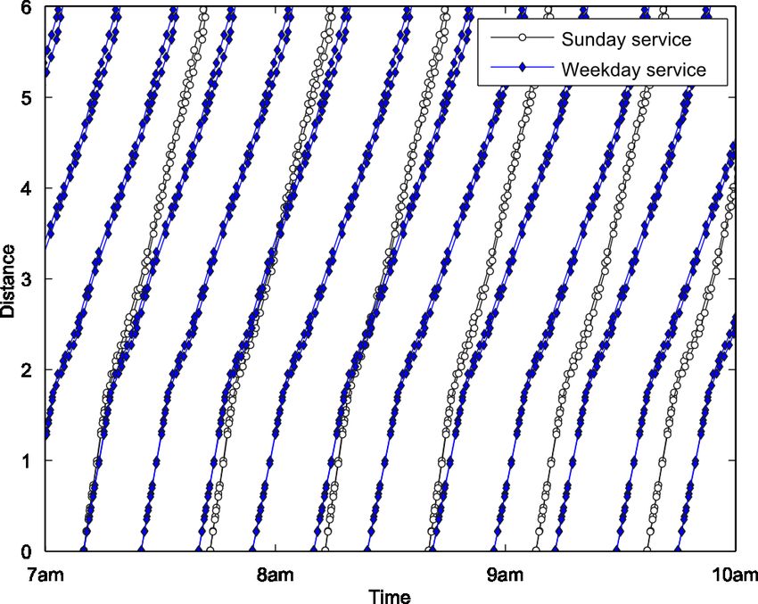
ABSTRACT
       A two-stage stochastic program that reoptimizes multi-modal transit schedules city-wide is pre-
       sented. The model works by perturbing or offsetting the schedule such that the expected value of
       waiting times at all transfer points in the system is minimized. Probabilistic information on trans-
       fers is gathered from a prototypical journey planner, a public-facing tool that transit riders query to
       find optimal paths through a multi-modal network. Aggregating journey plans in this manner pro-
       vides information on optimal transfers as perceived by the service operator, which are then targeted
       for improvements. The model is implemented on the large-scale transit network of Washington,
       D.C., where sampled journey plans representing 9% of the daily transit demand is employed to
       generate a modified schedule that leads to a reduction in passenger wait times by 26.38%. The re-
       sults serve to demonstrate how operators can take a user-centric view of their system as a fabric of
       services, gain insights from user interaction, and achieve no-cost improvements from coordinating
       services while accounting for uncertainty.

TRB 2013 Annual Meeting                                                             Paper revised from original submittal.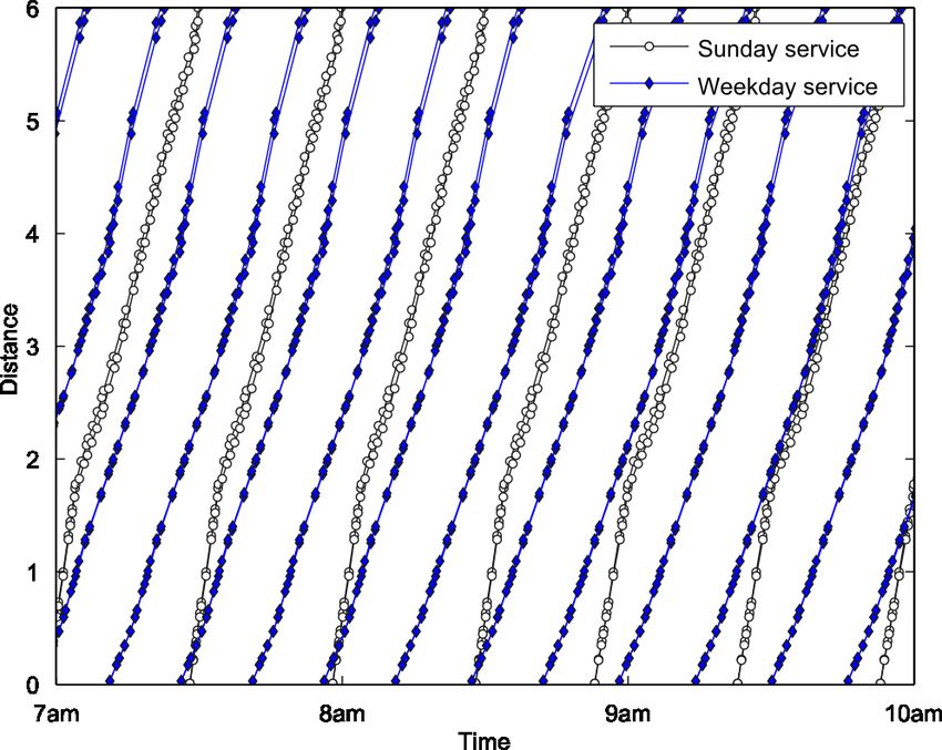
Nair, Coffey, Pinelli, Calabrese                                                                       2

       INTRODUCTION
       A two-stage stochastic program that reoptimizes multi-modal transit schedules city-wide is pre-
       sented. The model works by perturbing or offsetting the schedule such that the expected value of
       waiting times at all transfer points in the system is minimized. Information on transfers is gathered
       from a prototypical journey planner, a public-facing tool that transit riders query to find optimal
       paths through a multi-modal network. Transfer volumes of users across space and time are ag-
       gregated based on the result of queries that users make to a journey planner and are known only
       probabilistically.
               Aggregating journey plans in this manner provides information on optimal transfers as
       perceived by the service operator, which are then targeted for improvements. These transfers
       represent the ‘best-case’ service offerings on part of the operator, or a group of operators. While
       users may not necessary follow travel itineraries suggested by the journey planner, a representative
       sample of journey plans reveal systematic delays that occur at transfer points. The journey planner
       output, in essence, is the service that operators seek to provide.
               The use of a journey planner to assign users to paths in the network can be viewed as being
       analogous to an all-or-nothing assignment (a procedure where all users are assumed to take the
       shortest path to their destinations) but has key differences to that and other classical assignment
       procedures. A collection of journey planning requests constitute revealed or intended demand for
       travel. A collection of journey results constitute the operator’s best supply offerings. Since journey
       planners typically account for user preferences only in a very limited manner, heterogeneity in
       preferences (cost and travel time trade-offs for example) are ignored. Thus the principles of traffic
       assignment where supply and demand interact are not applied. Rather, the system is viewed entirely
       from the supply perspective. Given that operators supply journeys to a population of users, what
       are necessary schedule adjustments to provide optimal service?
               Existing transit schedules for large multi-modal transit networks typically evolve over the
       long term, and operators may lack a high-level snapshot of how interconnected services are em-
       ployed by the traveling public. Further, for the case of multi-modal networks, where different
       entities manage modes, the coordination may be hindered by organizational barriers (1). The aim
       of this work is to serve as a feedback loop within this overall transit planning process (2).
               There is considerable literature on schedule generation, schedule coordination and opti-
       mization for public transit networks. In a review paper, Guihaire and Hao (3), highlight the need
       for multi-modal considerations in transit planning and service coordination. For the purposes of
       this paper we focus on previous work that address the problem of aligning different services to
       minimize transfer time. Several works that have studied coordination of services (4, 5, 6) aim to
       coordinate arrivals of services at a single stop. Salzborn (7) presented rules to generate schedules
       for simple cases and Bookbinder and Désilets (8) considered the problem of minimizing waiting
       times when travel time between stops is random and services have fixed headways. Given the
       computational intractability of associated problems, several authors have used meta-heuristic ap-
       proaches to solve the general problem of transit schedule optimization (9, 10, 11, 12, 13, 14, 15, 16)
       using methods such as genetic algorithms, tabu search, intelligent agent based optimization, local
       search, or a combination of approaches (17). Specialized heuristics have been proposed as well,
       such as Lagrangian-based methods that seeks to optimize one line at a time (18) or generate a joint
       route and schedule plan (19). Large-scale network design and evaluations have been proposed
       for Rome (15), Boston (20), London (1), and Miami-Dade County (21). Liebchen (22) presents
       results from optimizing Berlin’s subways using a periodic event scheduling model where shorter

TRB 2013 Annual Meeting                                                            Paper revised from original submittal.
Nair, Coffey, Pinelli, Calabrese                                                                         3

       wait times are achieved using fewer trains.
                Some previous works have studied the stochastic nature of the transit optimization and its
       associated processes. Yan et al. (19) present a joint route-timetable design model that considers
       stochasticity in demand. Mesa et al. (23) aim to find robust fleet assignments such that frequencies
       on lines that face high demand are increased in a tactical manner. The model doesn’t consider
       stochasticity explicitly, but aims to find plans that robust against perturbation in demand. Includ-
       ing variability in problem inputs complicates problem design and solution approaches, given the
       combinatorial aspect of the decision variables. Liebchen and Stiller (24) seek timetables that are
       resistant to delays.
                The proposed work shares the spirit of work by Guo and Wilson (1) where the cost of trans-
       fer inconvenience is evaluated in London using a path choice model and focuses on a set of 303
       transfer movements. They highlight the importance of paying attention to transfer penalties that
       multi-modal transport systems impose on users along with barriers to reducing transfer penalties.
       There are significant institutional issues, since different portions of the network are managed by
       different entities, who each may view their role as being limited in correcting asynchronous sched-
       ules. The study also points to the gap in tools available to planners in quantifying and assessing
       the magnitude of transfer penalties, a gap that this paper seeks to address. In previous work by the
       authors (25), the multimodal connectivity of a transit system was analyzed and a hierarchy of trans-
       fers determined for different modal combinations. The paper proposed a deterministic program to
       optimize a single route, as opposed to a stochastic, system-wide method taken in this paper.
                The approach presented herein differs from the previously studied models in the follow-
       ing ways. Using journey planning queries and results, transfer costs city-wide are quantitatively
       characterized. This characterization leads to a model that determines local changes in schedule,
       defined by the offset, such that globally there is a decrease in expected waiting time. Key elements
       that have been the target of previous system optimization efforts such as frequencies, routes, and
       travel times, are retained from the existing schedule. The model is considered strategic, in that
       operational issues such as uncertainties in travel times and variability in demand are not consid-
       ered. The existing schedule is assumed to have adequate slack built in the travel times to absorb
       these uncertainties. The model keeps these slacks and existing travel time, but only seeks and opti-
       mal temporal shift, should one be available. The aim therefore is to remedy particularly egregious
       transfer delays, as identified by the trip plans. Additionally, any transfers that are currently possible
       and reflected in the trip planning sample is retained in the modified schedule. The high fidelity of
       journey plan data is leveraged to tune the schedule in a way that has not previously been feasible.
                The paper makes the following contributions. First, it provides a framework to operators to
       leverage journey planning information to provide a comprehensive view of how services are being
       offered. Second, it presents a stochastic model to optimize the schedules and suggest trip offsets
       such that expected waiting time is minimized. Third, it presents a large-scale implementation for
       Washington, D.C. using the Open Trip Planner (OTP) to generate a modified schedule for a typical
       Wednesday.
                The next section describes the two-stage optimization model in greater detail, followed by
       which the system in Washington, D.C. is described. The journey planner set up and query samples
       are presented next followed by an evaluation of the improved schedule.

TRB 2013 Annual Meeting                                                              Paper revised from original submittal.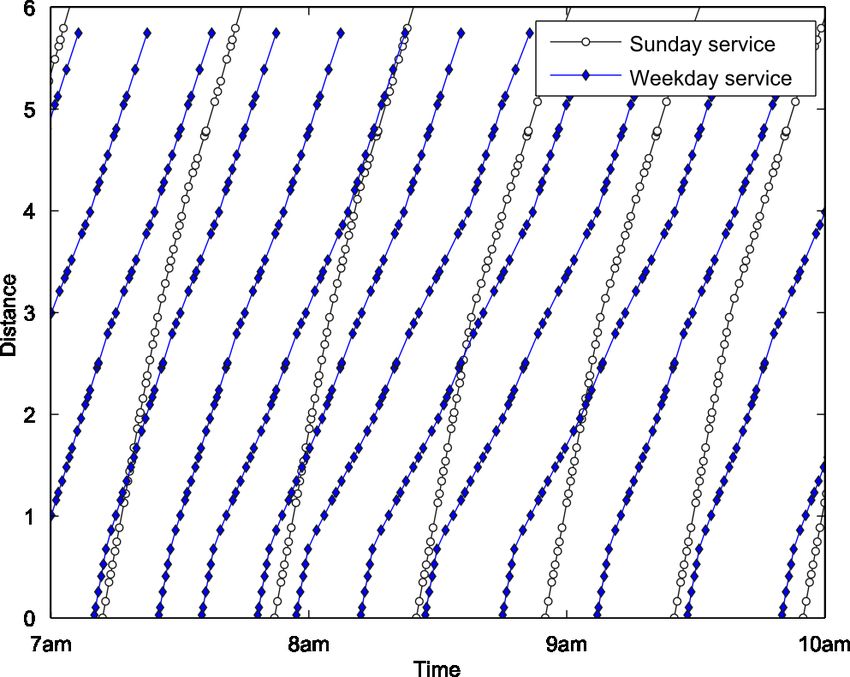
Nair, Coffey, Pinelli, Calabrese                                                                         4

       PROBLEM FORMULATION
       To clarify presentation of ideas, we use the following terminology which mirrors the General
       Transit Feed Specification (GTFS). The term route describes one transit service that serves a series
       of stops (e.g., Route 86). A route is made up of a collection of trips, where each trip represents
       one run of the route (e.g., 7:49am service of Route 86). A journey refers to a travel itinerary from
       the perspective of the user, and involves a set of trips and is the output of a journey planner (e.g.
       take 7:49am service of Route 86 till Stop b, and walk 10 minutes). A schedule describes the arrival
       and departure times of each trip at each stop along the route. While the route provides a spatial
       context, the trip information provides a spatio-temporal sense of the transit network. Transfers of
       passengers occur on this spatio-temporal network.
                Given (a) an existing schedule of a multimodal transit network, (b) a set of routes that need
       to be coordinated, (c) time headways for each trip for the route, (d) a representative set of user
       journey plans and (e) a probabilistic estimate of transfer volumes, we seek to find an optimal offset
       of each transit trip, such that the expected waiting times are minimized. The problem is strategic
       in nature, and the output is a modified schedule that aims to coordinate trips in a manner that users
       transferring at various points across the network experience minimal delays.
                In determining the optimal offset for each trip, the aim is to seek local improvements in
       departure time at terminal stations. Existing transfer opportunities are preserved, as are the number
       of trips for each route, frequency, and travel times between stops. Travel times between stops in the
       existing schedule are assumed to account for slack, variability in traffic conditions, and incorporate
       time-of-day and day-of-week effects. For large transit networks, where schedules are periodically
       modified and evolve to match existing conditions on the ground, planners are cognizant of service
       performance. The travel time estimates contained in the existing schedule are therefore valuable.
       As an example see Figure 2 for Washington, D.C. that shows the space-time diagrams for selected
       routes demonstrating the sensitivity of schedules to day-of-week effects. The model therefore
       seeks to preserve the travel time estimates.
                The model is defined on a general service network defined by a set of nodes N which
       represent stops, indexed by i. On this network, there are a set of trips Q indexed by p. Each trip p
       visits a subset of nodes Np . The service p arrives at node i at tpi . Each time a trip p arrives at stop
       i, users are presented with a set of transfer opportunities. Users transfer from and to trip p. Denote
       a set Q− pi as a set of trips that users seek to connect to (the minus sign signifies that they deboard
       trip p) and a set Q+  pi as a set of trips that users seek to connect from (the plus sign signifying that
       users board trip p). Each transfer opportunity has an associated volume of passengers that is only
                                                    −            +
       known probabilistically denoted by Cpqi        (ξ) and Cpqi (ξ) depending on if users deboard or board
       from service p to service q at node i. Here, ξ denotes the uncertainty in second-stage problem
       input. The service network and associated notation is shown in Figure 1. Define ∆pqi as the
       minimum transfer time required to make a successful transfer at node i from service p to q, and
       hp as the time headway of trip p. Additionally, define a and b as parameters that serve to bound
       perturbation as a fraction of time headway. For example, for values of a = −0.5 and b = 0.5, a
       trip is bound within one time headway of its existing departure.
                There are two sets of decision variables. From the operator perspective, denote xp , p ∈ Q
       as the time offset for each trip. This offset is determined by waiting times experienced by users,
       which are uncertain. Denote wpi (xp , ξ) as the waiting time in passenger-minutes associated with
       trip p at stop i. With these definitions, the network-wide transit coordination problem can be
       expressed as a two-stage stochastic program as follows.

TRB 2013 Annual Meeting                                                              Paper revised from original submittal.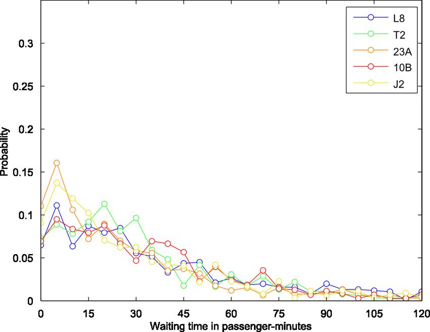
Nair, Coffey, Pinelli, Calabrese                                                                                 5

                    FIGURE 1 Service Network Representation and Associated Notation

                                         min Eξ [Q(xp , ξ)]                                                           (1)
                                          x
                           s.t.     ahp ≤ xp ≤ bhp                                                   ∀p ∈ Q           (2)
                    [(tqi + xq ) − (tpi + xp )] ≥ ∆qpi                         ∀p ∈ Q, q ∈   Q−
                                                                                              pi ,    i ∈ Np          (3)
                    [(tpi + xp ) − (tqi + xq )] ≥ ∆pqi                         ∀p ∈ Q, q ∈   Q+
                                                                                              pi ,   i ∈ Np           (4)
                                                xp ∈ R                                           ∀p ∈ Q,              (5)

       where Q(xp , ξ) is the second-stage program defined by

                                                XX
                          Q(xp , ξ) = min                   wpi (xp , ξ)                                              (6)
                                           w
                                                p∈Q i∈Np
                                       X
                                                                           −
             s.t.    wpi (xp , ξ) ≥           [(tqi + xq ) − (tpi + xp )] Cpqi (ξ)+
                                      q∈Q−
                                         pi
                                               X
                                                                                   +
                                                      [(tpi + xp ) − (tpi + xp )] Cpqi (ξ)     ∀p ∈ Q, i ∈ Np         (7)
                                              q∈Q+
                                                 pi

                                      wpi (xp , ξ) ∈ R+                                        ∀p ∈ Q, i ∈ Np         (8)

               Equation (1) is the first-stage objective to minimize the expected waiting times of passen-
       gers system-wide. Constraints (2) bounds the perturbation for each trip within a fraction of the
       time headway specified by parameters a and b. Constraints (3) and (4) serve to preserve transfers
       that passengers make to deboard and board respectively. Constraints (5) specify the time offset to
       be real. The second-stage model is defined over the distribution of uncertain transfer volumes ξ.
       The objective in Equation (6) is to minimize the waiting time system-wide. Constraint (7) specifies
       the waiting time in passenger-minutes to be the sum of waiting times for passengers to deboard
       and board. Constraint (8) restricts the wait times at all stops to be non-negative.
               The second-stage program is convex and always feasible if the support of the distribution
       of transfer volumes is finite. If empirical distributions are employed, then this is always the case,

TRB 2013 Annual Meeting                                                                      Paper revised from original submittal.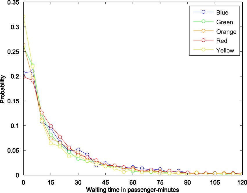
Nair, Coffey, Pinelli, Calabrese                                                                         6

       since the transfer volume is always finite. The program is also bounded below, since waiting times
       are non-negative. This can be exploited in the solution approach, as shown in the next section.
               The output schedule of the proposed model could potentially cause routes to have irregular
       service, since the time headways of the trips that make up a route are not equalized. While the
       extent of the irregularity can be controlled by changing the parameters a and b, there are inherent
       trade-offs between the costs and benefits of having an irregular schedule. Irregular services are
       detrimental to users who do not have transfers and arrive at stops without prior knowledge of the
       schedule. The expected wait times for such users increase on account of service irregularity. This
       added cost is as a result of aiming to improve services at portions of the network where there
       is significant transfers and usage. Some of the negative impacts can be ameliorated if changes
       in the regularity are conveyed to users ahead of time, or via real-time updates. This also places
       greater import on the way that transfer information is gathered, its accuracy, and distributional
       assumptions. The model also treats the set of transfers as being known. While there are methods
       from crowd-sourced data on trips, to numerical transit assignment procedures, that reveal a vast
       majority of transfers being made, there may be transfers that are not captured. This set of unknown
       transfers can potentially be worse off when left out of the model. The proposed model also retains
       any sub-optimal scheduling decisions that were in the existing schedule.

       Solving the Coordination Problem
       The solution technique is briefly described. One method to solve a two-stage stochastic program
       is to build a discrete set of scenarios that accurately depict the underlying distributions, termed
       the deterministic equivalent. The deterministic equivalent, has an underlying L-shaped matrix that
       can be solved using decomposition techniques. Methods such as those proposed by Van Slyke and
       Wets (26) and Birge and Louveaux (27, 28) can be used to solve the program. To generate the
       deterministic equivalent, the random vectors in the problem are assumed to be realized at certain
       values and associated probabilities. The continuous expectation function and the second-stage
       program can therefore be expressed as a series of linear programs. If the transfer volumes are
       discretized into a finite set of scenarios S, indexed by s, that occur with probability ps , then the
       objective (1) can be written as
                                               X XX
                                           min     ps         wpi (xp , ξˆs ),                           (9)
                                           x,w
                                                 s∈S   p∈Q i∈Np

       where, ξˆs is the realization of the random vector in scenario s. The value of transfer volumes in
                                                              − ˆ           + ˆ
       constraints (7) can be replaced with the realization Cpqi (ξs ) and Cpqi (ξs ) to yield the deterministic
       equivalent.

       LARGE-SCALE IMPLEMENTATION
       The major transit operator in the Washington, D.C. region is the Washington Metropolitan Area
       Transit Authority (WMATA). WMATA operates a multi-modal system consisting of a subway sys-
       tem, called Metrorail, and a bus system, called Metrobus. The system is extensive attracting 1.1
       million journeys on a typical workday that are served by 311 routes (not all operated by WMATA),
       that include 5 major Metrorail lines, serving 11,508 stops across the region. If each run of ev-
       ery route is aggregated, on a typical weekday, the system accounts for 24,390 trips, with a lower
       number of trips on Saturday (12,964 trips) and Sunday (9,935 trips). The system is a critical com-
       ponent of the urban mobility in the nation’s capital. WMATA has embraced open-data initiatives

TRB 2013 Annual Meeting                                                              Paper revised from original submittal.
Nair, Coffey, Pinelli, Calabrese 7
by releasing schedule information in the GTFS format, and providing a real-time Application Pro-
gramming Interface (API) that serves information on all aspects of the system. These efforts have
enabled this study.
The existing transit schedule has several service characteristics that are important and need
to be retained though any reoptimization efforts. A critical aspect of service is the sensitivity of
trip travel times to day-of-week effects and time-of-day effects. Since Washington, D.C. ranks
fourth in the nation in traffic congestion, such sensitivity is vital to generate realistic schedules.
Figure 2 graphically demonstrates the day-of-week effects for four sample routes. The slope of the
space-time trajectories represent the speed of the vehicles. The weekend schedules can be clearly
seen to have faster service, on account of traffic conditions. Similar trends are present, albeit less
drastic, for time-of-day effects.
(a) Route 54 (b) Route 90 with two variants
(c) Route 92 with two variants (d) Route B2
FIGURE 2 Sample Space-Time Trajectories of Bus Routes Showing Sensitivity to Traffic
Variations
WMATA also operates its own journey planner service on its website, while through its
public data efforts, journey planning is also possible through other widely used tools, such as
Google Maps and Microsoft Bing. For this study, data on journey planning requests made to these
TRB 2013 Annual Meeting Paper revised from original submittal.Nair, Coffey, Pinelli, Calabrese 8
services were not readily available, therefore a representative sample of journeys were sampled
based on transit demand for the region and the Open Trip Planner (OTP) employed using Open
Street Map (OSM) network data.
(a) Transit Demand Origins (darker = higher) (b) Transit Demand Destinations (darker = higher)
(c) Sample of Trip Origins (d) Sample of Trip Destinations
FIGURE 3 Spatial Patterns of Transit Demand and 9% Trip Sample
Transit Demand
Demand for transit is estimated by the regional travel demand model maintained by the Metropoli-
tan Washington Council of Governments (MWCOG). The model uses surveys and observed tran-
sit ridership numbers to calibrate and estimate mode choice models for the region. For a typical
workday, 1.1 million transit journeys are undertaken in the region. Based on this aggregated travel
TRB 2013 Annual Meeting Paper revised from original submittal.Nair, Coffey, Pinelli, Calabrese 9
pattern, a 9% sample, representing roughly 100,000 individual journeys, was constructed.
The aggregate daily transit trips are shown by origin (Figure 3(a)) and destination (Figure
3(b)). The constructed sample, shown in Figures 3(c) and 3(d) show the spatial dissaggregation of
trips. The sample is spatially representative of overall transit flows.
To derive an accurate temporal representation of usage, a temporal profile was used to
distribute the queries across time of day. The temporal profile is based on highway volume data
for a typical weekday in the region and follows the typical double-hump observed in a variety of
mobility processes. The temporal sample is therefore not representative, but indicative of overall
trends.
Transit Supply
To represent the transit supply side of the equation, open schedule data from WMATA, and the
street network from Open Street Maps (OSM) (29), were used to build a service network using
the Open Trip Planner (OTP) (30). Using open tools and data sources allows replication of our
proposed work across cities. The network and the journey planning engine available in OTP was
set up on an internal server. Using a Python script, OTP planned journeys for the 100,000 sampled
journeys.
For multi-modal trips there are several parameters that can be set, including maximum walk
time, maximum number of transfers, and restrictions on modal alternatives (e.g., bus-only, etc.).
All journeys were set to having the same parameters, i.e. user heterogeneity is ignored. Walk
distances are limited to 1/2 mile, maximum number of transfers allowed was set to five, and the
quickest path was sought. The trip start time was set based on the temporal profile sampled above.
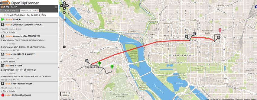
OTP returns several alternate itineraries, and only the fastest journey was considered. Figure 4.2
shows a example journey plan.
FIGURE 4 An Example Multimodal OTP Query Result Containing Three Modes: Walk,
Metrorail and Metrobus
There are some limitations in representing the true transit supply process. A main limitation
is the lack of support for journeys that involve a park-&-ride facility, when transit journeys are
considered. These facilities play an important role in providing transit access for suburban regions.
Secondary access modes such as bicycles and shared-bicycles were also not considered. Cost
criteria were not optimized in the travel journeys. Since metrorail is quicker but more expensive
for longer journeys than metrobus, journeys that have both options available will favor metrorail.
TRB 2013 Annual Meeting Paper revised from original submittal.Nair, Coffey, Pinelli, Calabrese 10
(a) System-wide Wait Times (b) Wait Times in Downtown Region
FIGURE 5 Spatial Distribution of Wait times
While these limitations don’t impact the in-system journey plans, they do alter the routes proposed.
The limitations can be overcome if the journey planner incorporates these factors. With the a set
of synthesized journey requests and a network representation of the transit supply process, transfer
costs system-wide can be calculated.
Estimating Transfers
The resulting journey plans from OTP are parsed and transfer information recorded for multi-leg
journeys. Transfers occur in two modes. Waiting transfers refer to changes from one service to
another. Walking transfers involve a change in service and a walk to the next service. Both types
of transfers are translated to waiting time, since our purpose is to adjust the schedule. So the walk
component of transfers is simply added to ∆pqi , the minimum time needed to transfer at stop i
between services p and q. A detailed characterization of the transfer process is presented in Coffey
et al. (25).
A total of 59,344 unique transfer movements were captured from the sample. Each transfer
movement represents a service pair at a point in space and time. Two key performance metrics are
employed to convey wait times. The basic measure is the wait time in minutes of each transfer,
as represented by the journey plan. The second is a volume-weighted waiting time metric in
passenger-minutes that is derived by equally apportioning the total travel demand for an origin-
destination pair among all journey plans for that pair.
First, an aggregate picture of waiting times is presented. Figure 5 shows the spatial dis-
tribution waiting time across the network. Assuming a representative sample, a total of 26,392
passenger-hours of delay was measured for a typical weekday. Assuming a value-of-time (VOT)
of $18 per hour, the estimated cost of these wait times is $475,059 daily.
The distribution of wait times by route can be examined to evaluate if there is a high oc-
currence of particularly extreme waits. Figure 6 show the wait time distribution for selected routes
differentiated by mode, showing the higher level of service of metrorail leading to lower wait times.
TRB 2013 Annual Meeting Paper revised from original submittal.Nair, Coffey, Pinelli, Calabrese 11
From a transfer perspective, there is a small proportion of journeys that experience high transfer
times that are then optimized. If wait times are aggregated by route, across time and space, route
performance can be measured. Figure 7 shows the top twenty routes in terms of daily delay. The
major metrorail services that are high volume and frequent, account for significant wait times in-
curred by passengers. The improvements in wait times based on the modified schedule are also
shown.
(a) Metro-rail routes (b) Metro-bus routes
FIGURE 6 Distribution of wait Times for Different Services
REOPTIMIZATION RESULTS
The schedule reoptimization model was solved using CPLEX and a modified weekday schedule
generated for the entire network. Computational details are omitted for brevity, except to note
that 100 scenarios were considered for the second-stage model, where the transfer volumes were
assumed to be log-normal, with the mean equal to the transfer volume estimated from the sample.
The wait times for the 9% sample were recomputed, assuming users would have been
offered the same journey plans. System-wide waiting time based on the modified schedule were
computed at 19,429 passenger-hours (or $349,722 assuming a VOT of $18/hour). This represents
a 26.38% improvement in system-wide wait times, achieved by the schedule offset.
The improvements in wait times were disaggregated by route for which passengers wait to
board. Figure 7 shows the reduction in wait times as a result of the modified schedule. These are
reported for the top 20 routes with largest wait times in passenger-minutes based on the existing
schedule.
The schedule modifications for selected routes is plotted in Figure 8. The temporal offset
suggested by the model can be ascertained by comparing the existing and modified trajectories.
Since the a and b parameters were considered as −0.5 and 0.5, the offset is limited by one half
headway in either temporal direction as shown by Figure 9 which shows the offset distribution
for the entire city. This leads to some routes having irregular headways. One method to limit the
regularity is to change the a and b parameters, or introduce route specific parameters, after the
routes have been determined. Ongoing efforts seek to determine the route specific values for these
parameters automatically, such that routes are equalized.
Since the model weights the wait times by passenger volumes while seeking the correction,
TRB 2013 Annual Meeting Paper revised from original submittal.Nair, Coffey, Pinelli, Calabrese 12
FIGURE 7 Wait Times to Board Route Before and After Schedule Adjustment
there are a small proportion of users that see reduced service. The reason this occurs is because the
temporal offset optimizes for nodes where transfer volumes are greater, at the expense of nodes at
which volumes are low. The distribution of transfer volumes can be compared before and after the
schedule update to see what fraction of users see a decreased service as shown in Figure 10. The
decreased service is experienced by approximately 15% of users. However the magnitude of the
decrease is significantly lower than the magnitude of the improvements seen for the majority of
users.
CONCLUSIONS
A stochastic program that computes optimal time offsets for a large-scale transit network is im-
plemented for Washington, D.C. Using output of a journey planner, the transfer penalties, in terms
of wait times, that multi-modal networks impose on users is characterized. The high fidelity with
which journey plans depict itineraries, coupled with the large volume of queries that agencies or
third party providers process, allow a rich characterization of transfers that then drive a system
improvement, in this case temporal offsets.
For Washington, D.C. based on a representative sample of queries, users wait a total of
26,392 passenger-hours. Using the proposed model to generate a modified schedule, the waiting
times are reduced by an estimated 26.38%. The wait times are also characterized by different
routes and distributions, providing vital performance metrics that could also be used to provide
system insights.
Extensions of the model that seek to provide equalized headways, include reliability in-
formation on routes and uncertainty in travel times, distinguish special event patterns from trip
queries would add value for transit operators. This methodology presented leverages information
gleaned from contact with users via a journey planner. With time, the set of requests are likely to
change to reflect changes in travel patterns. A periodic review of the schedule based on evolving
TRB 2013 Annual Meeting Paper revised from original submittal.Nair, Coffey, Pinelli, Calabrese 13
FIGURE 8 Comparison of Modified and Existing Schedules for Selected Bus Routes
TRB 2013 Annual Meeting Paper revised from original submittal.Nair, Coffey, Pinelli, Calabrese 14
FIGURE 9 Distribution of Offsets for Entire System
FIGURE 10 Distribution of Wait Times Difference
travel patterns can also provide a closer feedback loop to the design process.
A key concept of the proposed work is to have a representative sample of journey plans.
The sample should accurately reflect how transfers are conducted in the system, so that the re-
optimized schedule provides efficient mobility for all.
ACKNOWLEDGMENTS
The authors would like to thank Ron Kirby, Ron Malone, and Mary Martchouk at the Metropoli-
tan Washington Council of Governments for providing data on transit demand for the Washing-
ton, D.C. region. Cathal Coffey acknowledges support from the Strategic Research Cluster grant
TRB 2013 Annual Meeting Paper revised from original submittal.Nair, Coffey, Pinelli, Calabrese 15
(07/SRC/I1168) by Science Foundation Ireland, and an IBM Ph.D. Fellowship award.
REFERENCES
[1] Guo, Z. and N. Wilson, Assessing the cost of transfer inconvenience in public transport sys-
tems: A case study of the London Underground. Transportation Research Part A: Policy and
Practice, Vol. 45, No. 2, 2011, pp. 91–104.
[2] Ceder, A. and N. Wilson, Bus network design. Transportation Research Part B: Methodolog-
ical, Vol. 20, No. 4, 1986, pp. 331–344.
[3] Guihaire, V. and J.-K. Hao, Transit network design and scheduling: A global review. Trans-
portation Research Part A: Policy and Practice, Vol. 42, No. 10, 2008, pp. 1251–1273.
[4] Daganzo, C., On the coordination of inbound and outbound schedules at transportation ter-
minals. In International Symposium on Transportation and Traffic Theory, Yokohama-Shi,
Japan, 1990, pp. 379–390.
[5] Chowdhury, S. and S. Chien, Optimization of transfer coordination for intermodal transit
networks. In Transportation Research Board Annual Meeting, at Washington, DC, 2001.
[6] Ceder, A., B. Golany, and O. Tal, Creating bus timetables with maximal synchronization.
Transportation Research Part A: Policy and Practice, Vol. 35, No. 10, 2001, pp. 913–928.
[7] Salzborn, F., Scheduling bus systems with interchanges. Transportation Science, Vol. 14,
No. 3, 1980, pp. 211–231.
[8] Bookbinder, J. and A. Désilets, Transfer optimization in a transit network. Transportation
science, Vol. 26, No. 2, 1992, pp. 106–118.
[9] Ngamchai, S. and D. Lovell, Optimal time transfer in bus transit route network design using
a genetic algorithm. Journal of Transportation Engineering, Vol. 129, 2003, p. 510.
[10] Chakroborty, P., K. Deb, and P. Subrahmanyam, Optimal scheduling of urban transit systems
using genetic algorithms. Journal of transportation Engineering, Vol. 121, No. 6, 1995, pp.
544–553.
[11] Cevallos, F. and F. Zhao, Minimizing Transfer Times in Public Transit Network with Genetic
Algorithm. Transportation Research Record, Vol. 1971, No. 1, 2006, pp. 74–79.
[12] Liu, Z., J. Shen, H. Wang, and W. Yang, Regional Bus Timetabling Model with Synchroniza-
tion. Journal of Transportation Systems Engineering and Information Technology, Vol. 7,
No. 2, 2007, pp. 109–112.
[13] Shrivastava, P. and M. OŠMahony, Design of feeder route network using combined genetic
algorithm and specialised repair heuristic. Journal of Public Transportation, Vol. 10, No. 2,
2007, pp. 109–133.
[14] Blum, J. and T. Mathew, Intelligent Agent Optimization of Urban Bus Transit System Design.
Journal of Computing in Civil Engineering, Vol. 25, 2011, pp. 357–369.
TRB 2013 Annual Meeting Paper revised from original submittal.Nair, Coffey, Pinelli, Calabrese 16
[15] Cipriani, E., S. Gori, and M. Petrelli, Transit network design: A procedure and an application
to a large urban area. Transportation Research Part C: Emerging Technologies, Vol. 20, 2012,
pp. 3–14.
[16] Ibarra-Rojas, O. J. and Y. a. Rios-Solis, Synchronization of bus timetabling. Transportation
Research Part B: Methodological, Vol. 46, No. 5, 2012, pp. 599–614.
[17] Zhao, F. and X. Zeng, Simulated annealing–genetic algorithm for transit network optimiza-
tion. Journal of computing in civil engineering, Vol. 20, 2006, pp. 57–68.
[18] Castelli, L., R. Pesenti, and W. Ukovich, Scheduling multimodal transportation systems. Eu-
ropean Journal of Operational Research, Vol. 155, No. 3, 2004, pp. 603–615.
[19] Yan, S., C. Chi, and C. Tang, Inter-city bus routing and timetable setting under stochastic
demands. Transportation Research Part A: Policy and Practice, Vol. 40, No. 7, 2006, pp.
572–586.
[20] Guo, Z. and N. Wilson, Assessment of the Transfer Penalty for Transit Trips Geo-
graphic Information System-Based Disaggregate Modeling Approach. Transportation Re-
search Record: Journal of the Transportation Research Board, Vol. 1872, 2004, pp. 10–18.
[21] Zhao, F., Large-scale transit network optimization by minimizing user cost and transfers.
Journal of Public Transportation, Vol. 9, No. 2, 2006, p. 107.
[22] Liebchen, C., The First Optimized Railway Timetable in Practice. Transportation Science,
Vol. 42, No. 4, 2008, pp. 420–435.
[23] Mesa, J., F. Ortega, and M. Pozo, Effective Allocation of Fleet Frequencies by Reducing
Intermediate Stops and Short Turning in Transit Systems. Robust and Online Large-Scale
Optimization, 2009, pp. 293–309.
[24] Liebchen, C. and S. Stiller, Delay resistant timetabling. Public Transport, Vol. 1, 2009, pp.
55–72, 10.1007/s12469-008-0004-3.
[25] Coffey, C., R. Nair, F. Pinelli, and F. Calabrese, Missed Connections: Quantifying and Opti-
mizing Multimodal Interconnectivity in Cities. Submitted, in review.
[26] Van Slyke, R. and R. Wets, L-shaped linear programs with applications to optimal control
and stochastic programming. SIAM Journal on Applied Mathematics, 1969, pp. 638–663.
[27] Birge, J. and F. Louveaux, A multicut algorithm for two-stage stochastic linear programs.
European Journal of Operational Research, Vol. 34, No. 3, 1988, pp. 384–392.
[28] Birge, J. and F. Louveaux, Introduction to stochastic programming. Springer Verlag, 1997.
[29] Open Street Maps. http://www.openstreetmap.org/, 2012.
[30] Open Trip Planner. http://opentripplanner.com/, 2012.
TRB 2013 Annual Meeting Paper revised from original submittal.You can also read