Water Resource Systems Analysis for Water Scarcity Management: The Thames Water Case Study - MDPI
←
→
Page content transcription
If your browser does not render page correctly, please read the page content below
water
Article
Water Resource Systems Analysis for Water Scarcity
Management: The Thames Water Case Study
Mark Morley 1         and Dragan Savić 1,2, *
 1   KWR Water Research Institute, 3433 PE Nieuwegein, The Netherlands; mark.morley@kwrwater.nl
 2   Centre for Water Systems, College of Engineering, Mathematics and Physical Sciences, University of Exeter,
     Exeter EX4 4QF, UK
 *   Correspondence: dragan.savic@kwrwater.nl or d.savic@exeter.ac.uk

 Received: 17 May 2020; Accepted: 18 June 2020; Published: 20 June 2020

 Abstract: Optimisation tools are a practical solution to problems involving the complex and
 interdependent constituents of water resource systems and offer the opportunity to engage with
 practitioners as an integral part of the optimisation process. A multiobjective genetic algorithm
 is employed in conjunction with a detailed water resource model to optimise the “Lower Thames
 Control Diagram”, a set of control curves subject to a large number of constraints. The Diagram is
 used to regulate abstraction of water for the public drinking water supply for London, UK, and to
 maintain downstream environmental and navigational flows. The optimisation is undertaken with
 the aim of increasing the amount of water that can be supplied (deployable output) through solely
 operational changes. A significant improvement of 33 Ml/day (1% or £59.4 million of equivalent
 investment in alternative resources) of deployable output was achieved through the optimisation,
 improving the performance of the system whilst maintaining the level of service constraints without
 negatively impacting on the amount of water released downstream. A further 0.2% (£11.9 million
 equivalent) was found to be realisable through an additional low-cost intervention. A more realistic
 comparison of solutions indicated even larger savings for the utility, as the baseline solution did not
 satisfy the basic problem constraints. The optimised configuration of the Lower Thames Control
 Diagram was adopted by the water utility and the environmental regulators and is currently in use.

 Keywords: water resource modelling; multiobjective optimisation; river abstraction

1. Introduction
      The field of systems analysis has often been associated with the advent of operations research
during and after the Second World War, while its application to water resource systems advanced
more significantly from around the 1970s, when computers became widely available [1]. The parallel
development in computational hydraulics and hydrology, which was also stimulated by the advent of
modern information and communication technology, led to the emergence of the aligned discipline
of hydroinformatics in the 1990s [2]. Both systems analysis and hydroinformatics embrace not only
technological issues, such as scientific methods and the application of data, models and decision support
tools, but also much wider questions of the role of the discipline in addressing societal challenges [2].
Water security, resilience, governance and ethical issues are just a few of those societal challenges
that are also affected by growing climate, population and uncertainty concerns. The complexity of
water issues, often involving incomplete, contradictory and changing requirements, together with the
involvement of stakeholders holding multiple and opposing views, give water challenges a “wicked”
(ill-defined) character [3,4]. The wicked nature of water resource challenges also meant that a multitude
of methods for optimising the planning and management of water resources developed over the
years [5,6] were not fully adopted in practice [7].

Water 2020, 12, 1761; doi:10.3390/w12061761                                        www.mdpi.com/journal/water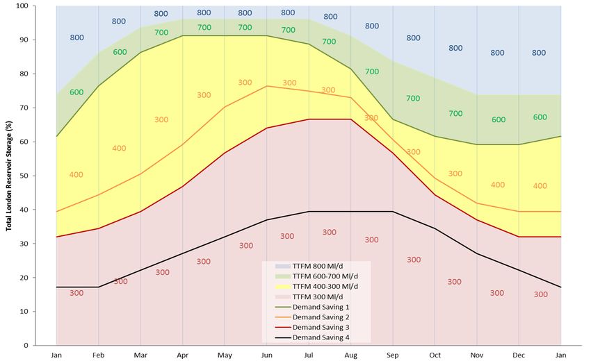
Water 2020, 12, 1761 2 of 10
One of the challenges most often encountered in water resource systems planning and management
is how to define operating rules for multiple sources requiring an integrated vision, thus accounting
for interrelations and interdependencies among complex system components [5–8]. The widespread
reporting of the use of simulation and optimisation methods shows that systems analysis tools are
being used in practice [8,9]. However, despite this vast wealth of literature, publications reporting on
practical applications of such tools, their impact and the experiences of analysts and clients are rare.
Each water service provider in England and Wales must produce a water resources management
plan (WRMP), which is updated every five years. Such plans aim to ensure “sufficient supply of water
to meet the anticipated demands of its customers over a minimum 25-year planning period, even under
conditions where water supplies are stressed” [10]. This paper presents a case study in which systems
analysis tools were used to develop a constituent of a WRMP for a water service provider, Thames
Water, considering the complexities and requirements of such a plan. An optimisation tool was
developed to redesign a key component of the water management strategy for the River Thames in
such a way as to maximise the capacity of the system to supply drinking water whilst ensuring the
maintenance of strict environmental criteria regarding the quantity of water left in the river as it flows
into its tidal reach.
2. Materials and Methods
Thames Water abstracts water from the lower reaches of the River Thames for the purpose of
public water supply via a number of large reservoirs to the west of London. Transfers are also made to
reservoirs in the Lea Valley found to the northeast of London. Left unconstrained, these abstractions
could have a deleterious effect on the downstream environment. Accordingly, these are undertaken in
agreement with the English Environment Agency (EA) environmental regulator, under Section 20 of the
Water Resources Act 1991 [11]. This agreement describes the Lower Thames Control Diagram (LTCD),
which is used to control the level of abstraction permitted as a function of current reservoir storage.
Thames Water seeks to optimise the LTCD, with a view to maximising the deployable output of the
system as a whole. Deployable output is considered to be the maximum output capacity (i.e., demand
that could be supplied) of one or more commissioned water sources that can achieve a prescribed
level of service as constrained by factors such as, inter alia, hydrological yield, licence constraints and
treatment and transport and pumping capacity.
In addition, a second optimisation scenario was evisaged in which aggregate could be extracted
from an existing reservoir to facilitate additional storage capacity for the system. This was to be run as
a separate analysis to determine what impact such a change would have on the deployable output of
the system as a whole.
2.1. Lower Thames Control Diagram
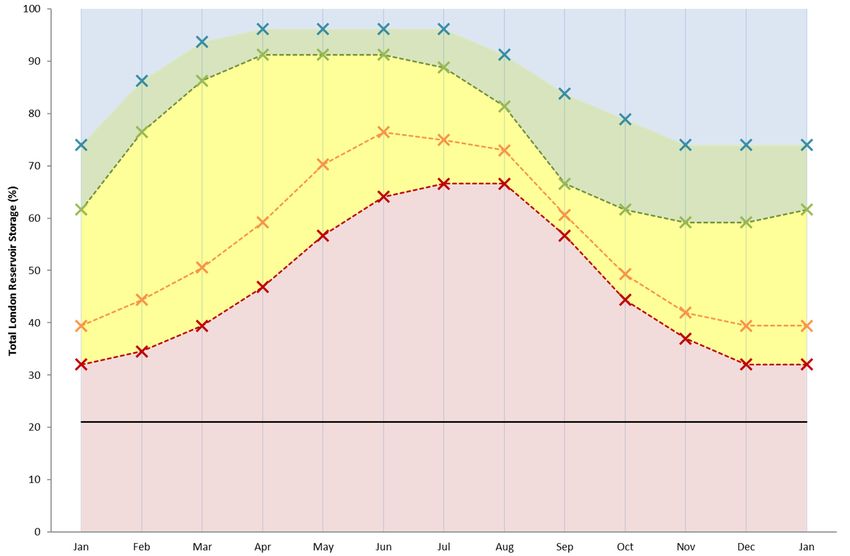
The LTCD controls abstraction principally by defining a target environmental and navigational
flow that must reach the tidal reaches of the Thames at Teddington Lock: the Teddington target flow (TTF).
The TTF matrix is illustrated in Figure 1 where each month/operating band has a minimum flow target.
As can be seen, when reservoir storage is full, Thames Water are obligated to ensure that a
minimum of 800 Ml/day is discharged into the tidal reach. This figure diminishes as reservoir storage
becomes lower, with the constraints becoming more relaxed in the late spring and early summer months.
The solid lines on the LTCD represent the points at which the various demand-saving measures,
agreed with the environmental (EA) and economic (Ofwat) regulators and outlined in the appropriate
act and statutory instruments [11,12], are implemented:
• Level 1: intensive media campaign.
• Level 2: sprinkler/unattended hosepipe ban and enhanced media campaign.
• Level 3: temporary use ban, ordinary drought order (non-essential use ban).
• Level 4: emergency drought order (e.g., standpipes and rota cuts).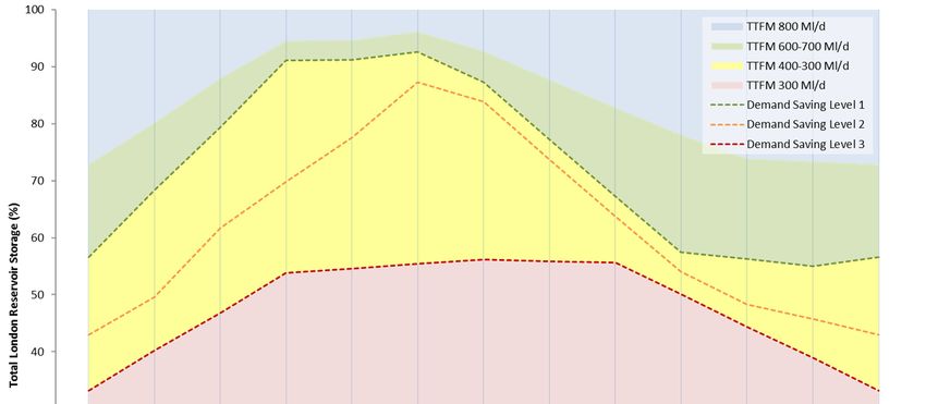
Water 2020, 12, 1761 3 of 10
Water 2020, 12, x FOR PEER REVIEW 3 of 11
Figure 1. The
Figure 1. The Lower
Lower Thames
Thames Control
Control Diagram
Diagram (LTCD).
(LTCD).
In
Asaddition,
can be seen,the “crossing” of these
when reservoir demand-saving
storage linesWater
is full, Thames also triggers the implementation
are obligated to ensure thatofa
further
minimum schemes,
of 800 such
Ml/dayas transfers of water
is discharged intofrom neighbouring
the tidal reach. Thiswater resource
figure zonesasand
diminishes the usestorage
reservoir of the
Thames Gateway desalination plant at Beckton [13].
becomes lower, with the constraints becoming more relaxed in the late spring and early summer
For the purposes of this analysis, the existing LTCD [14], which dates back to 1980 and was last
months.
updated
The in 1997,
solid is considered
lines on the LTCD torepresent
give a deployable
the pointsoutput of 2285
at which Ml/day.
the various The shape of the
demand-saving curves
measures,
was derived by iteratively applying a water resource model over the historical draw-down
agreed with the environmental (EA) and economic (Ofwat) regulators and outlined in the appropriate record and
adjusting the profiles
act and statutory to account
instruments for violations
[11,12], of the level of service constraints.
are implemented:
2.2. Constraints
• Level 1: intensive media campaign.
• The deployable
Level output (DO) is defined
2: sprinkler/unattended hosepipe asban
being
andtheenhanced
maximum demand
media that the system can supply
campaign.
•
whilst meeting
Level the termsuse
3: temporary of ban,
the level of service.
ordinary drought The level(non-essential
order of service criteria, measured over a time
use ban).
•
horizon of 100
Level years, agreed
4: emergency with order
drought the regulator for the system
(e.g. standpipes are:cuts).
and rota
• Level 1 events should occur at a frequency of no more than 1 in 5 years.
In addition, the “crossing” of these demand-saving lines also triggers the implementation of
•further
Level 2 events
schemes, should
such occur at of
as transfers a frequency
water from of neighbouring
no more than 1water
in 10resource
years. zones and the use of
•the Thames
Level 3 events should occur at a frequency of no
Gateway desalination plant at Beckton [13]. more than 1 in 20 years.
• Level 4 events
For the are of
purposes considered unacceptable
this analysis, and
the existing thus [14],
LTCD any solution mustback
which dates not allow such
to 1980 andan event.
was last
updated in 1997, isoccurrence
The permitted consideredoftoLevel
give 2a and
deployable outputisofcomplicated
Level 3 events 2285 Ml/day.byThe
the shape
impactofofthe
thecurves
Flood
and Water Management Act 2010 [15], which stipulates that there should be periods of 14 and 56record
was derived by iteratively applying a water resource model over the historical draw-down days
and adjusting the profiles to account for violations of the level of service constraints.
of public consultation, respectively, in advance of these measures being implemented. Accordingly,
it is required that 14 days elapse between a Level 1 and a Level 2 event starting, and 56 days between
2.2. Constraints
the start of Level 2 and Level 3 events. The existing LTCD DO of 2285 Ml/day did not consider these
additional constraints.output
The deployable As at (DO)
present, the linesasdefining
is defined being thethemaximum
implementation
demand of that
the demand-saving
the system can
levels
supplywere to be
whilst considered
meeting coincident
the terms of the with
level the boundaries
of service. between
The level the respective
of service criteria, TTF bands.over a
measured
timeFurther
horizon constraints
of 100 years,were agreed
agreed with with the environmental
the regulator regulator
for the system are: for the production of the
new LTCD, which included ensuring that the boundary between the TTF800 and TTF600-700 bands
• Levelblue
(coloured 1 events should
and green, occur at a frequency
respectively, in Figure 1)ofshould
no more than
be no 1 in 5than
higher years.
its current implementation.
• addition,
In Level 2 events should occur
the definition of theatLevel
a frequency
4 curveofisno more than
changed 1 in 10 years.
to represent 30 days of storage at the
• Level 3 events should occur at a frequency of no more than 1 in 20 years.
• Level 4 events are considered unacceptable and thus any solution must not allow such an event.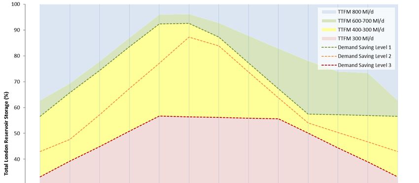
in subsequent generations in order to determine the maximum valid DO for the combination of curve
profiles specified. This was achieved by dynamically constraining the allowed range of the DO
decision variable. If a feasible solution was subsequently found to have a valid higher DO, then the
minimum value of the DO decision variable for this solution would be set to the new high DO.
Water 2020, 12, 1761                                                                                     4 of 10
Similarly, if the evaluation of a higher DO proved not to be feasible, then the maximum value of            the
DO would be pegged to that higher value, so that higher values could no longer considered for that
solution. Over
prevailing   DO and  time,
                        thusthe
                             thispopulation    of solutions
                                  line will represent        gradually
                                                      a greater          migrated
                                                                storage capacity fortohigher
                                                                                        theirdemand
                                                                                              true DO   values.
                                                                                                     scenarios;
“Immature”       solutions   whose   maximum     DO   has  yet to be determined   were   protected from
the revised form of the Level 4 curve for the baseline scenario is shown as the horizontal line in Figurebeing 2.
removed from the population.

           Figure 2. Annotated LTCD showing
                                    showing the
                                            the 48
                                                48 decision
                                                   decision variables
                                                            variables needed
                                                                      needed to
                                                                              to define
                                                                                 define its
                                                                                         its shape.
                                                                                             shape.

      The addition of each of these constraints increases the complexity of the problem to such an extent
that it is difficult to imagine an efficient mechanism for deriving a workable solution, let alone a good
one, without the use of optimisation tools.

2.3. Aquator Model
     As part of this research project, an Aquator [16] water resources model was made of the whole
Thames Water resource and supply area. Aquator is widely used in the UK water industry and has been
used as a platform for a software application: AquatorGA [17]. This optimisation tool has been used in
a number of projects in which it acts as a controller for the Aquator modelling package. The Aquator
model simulates the daily operation of the system, applying the rules and constraints of the LTCD.
Uncertainty in future inflows is accommodated by running the model for a given present-day DO
against historic inflow data from 1920 to 2010. These inflows could be substituted by stochastically
generated ensembles, if required. The model is executed by the optimisation algorithm repeatedly for
a given DO and curve profile combination and is used to determine whether the combination (a) is
feasible, and (b) meets the constraints of the maximum number of level of service events that occur in
each category over the 90-year time horizon. The model is able to operate in two modes: a simplified
cut-down model, for the purposes of optimisation, and a full mode, for validating the results as a
post-process, which takes approximately three times longer to run. Tests showed that the differences in
the accuracy of the two modes of the model were of the order of 1 or 2 Ml/day. Even so, the cut-down
model required around 1 h to run for the historic inflow data.

2.4. Genetic Algorithm Optimisation
     Genetic algorithms (GAs) are a powerful optimisation technique which can be applied to a wide
variety of problems without any prerequisite knowledge of the problem domain. They perform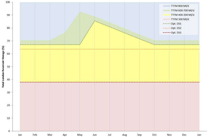
Water 2020, 12, 1761                                                                                5 of 10

a directed search of the decision space, which also contains a stochastic component, based on the
“survival of the fittest” principle. The methodology takes advantage of the simulation model, i.e.,
Aquator in this case, ensuring that each potential solution is tested using a realistic representation
of the water resource system being analysed. The most important advantage of GA over any other
optimisation techniques is its flexibility in simulating different decision variables, objectives and
constraints, due to the fact that any potential solution can be assessed directly in the model without
the need for the derivation of specific mathematical properties (e.g., linearity) or expressions (e.g.,
derivatives), which present the main drawbacks to classic optimisation methods. A multiobjective
GA [18] that can easily handle multiple constraints was used as part of the AquatorGA software.
     Two objectives were specified for the production of the new LTCD: to maximise the deployable
output of the system and to minimise the complexity of the produced curves in order to make them
acceptable to practitioners by reducing their jaggedness. Although this latter objective is, strictly
speaking, not a genuine operational requirement, this objective was included as a result of the
discussions with the client and consideration of the practicability of the implementation of the solution.
Past applications of the AquatorGA software demonstrated that practitioners find it easier to relate to
and explain control rules and curves when they are presented as smooth curves rather than more jagged
ones, even though these may be perfectly valid solutions and represent mathematically “better” results.
     The shape of the LTCD is represented by 48 decision variables representing the monthly values
for each of the four profile curves, as shown in Figure 2. Each variable was defined with a nominal
precision of 1 decimal place and was permitted to vary between the level of the Level 4 line and the
current boundary between the TTF800 and TTF600-700 bands. In order to accommodate the curve
complexity objective, each of the 48 curve shape decision variables was coupled with a Boolean decision
variable, which determined whether the point was considered as part of the curve or not. In this way,
by “switching off” the curve points, the optimisation can easily simplify the shape of the curves.
     One further decision variable was used to define the requested DO for the solution, hence the
unusual situation where the DO was both an objective a decision variable. This approach was adopted
because the total demand on the system was, along with the curve profile shapes, an input value
submitted to the Aquator simulation model. The long run-times of the Aquator model meant that
it was important that the number of infeasible solutions evaluated was minimised. To this end,
once a feasible set of profiles had been identified, the DO decision variable was gradually increased in
subsequent generations in order to determine the maximum valid DO for the combination of curve
profiles specified. This was achieved by dynamically constraining the allowed range of the DO decision
variable. If a feasible solution was subsequently found to have a valid higher DO, then the minimum
value of the DO decision variable for this solution would be set to the new high DO. Similarly, if the
evaluation of a higher DO proved not to be feasible, then the maximum value of the DO would
be pegged to that higher value, so that higher values could no longer considered for that solution.
Over time, the population of solutions gradually migrated to their true DO values. “Immature”
solutions whose maximum DO has yet to be determined were protected from being removed from
the population.
     The combination of decision variables and constraints gives rise to a solution space consisting
of 48 curve shape decisions, each of which can take on 1000 different values (0–100% at 1 decimal
place = 100048 options) plus 48 boolean decisions (248 options) plus a single integral decision variable
representing DO which is allowed to vary between 1800 and 2350 Ml/day (550 options), which gives
100048 × 248 × 550 = 1.5 × 10161 possible solutions to the problem. The use of a genetic algorithm
allowed this huge space to be efficiently sampled and evaluated, using of the order of 120,000 solutions.
Nevertheless, with each solution taking around 1 h to simulate on a high-specification PC (2015),
it was necessary to employ some form of parallelisation in order to reduce the optimisation run-times
to a manageable length. To this end, the AquatorGA software used in this optimisation included a
distributed-processing system in order to militate against the extended run-times that are a common
issue when optimising evolution algorithms applied to hydroinformatics problems. The software
this huge space to be efficiently sampled and evaluated, using of the order of 120,000 solutions.
Nevertheless, with each solution taking around 1 hour to simulate on a high-specification PC (2015),
it was necessary to employ some form of parallelisation in order to reduce the optimisation run-times
to a manageable length. To this end, the AquatorGA software used in this optimisation included a
distributed-processing system in order to militate against the extended run-times that are a common
Water 2020, 12, 1761 6 of 10
issue when optimising evolution algorithms applied to hydroinformatics problems. The software
employs the industry standard message passing interface (MPI) protocol to execute many Aquator
simulation
employs the models in parallel.
industry standardThis systempassing
message permitsinterface
the concurrent evaluation
(MPI) protocol of a large
to execute number
many of
Aquator
potential solutions
simulation models either on local This
in parallel. processors
systemorpermits
to otherthe
computers
concurrent onevaluation
a local areaofnetwork.
a large number of
For the purposes of this optimisation, the software was deployed across
potential solutions either on local processors or to other computers on a local area network. a cluster of five
workstations, each equipped with two Intel Xeon E5645 CPU packages, which
For the purposes of this optimisation, the software was deployed across a cluster comprise six cores
of five
running at 2.4 GHz
workstations, eachforequipped
a total ofwith
60 processor
two Intelcores.
XeonInE5645
addition,
CPUthis hardware
packages, architecture
which comprisecan sixtake
cores
advantage of hyper-threading technology, which improves the performance of identical
running at 2.4 GHz for a total of 60 processor cores. In addition, this hardware architecture can threads
running on multiple
take advantage cores by around technology,
of hyper-threading 10%–20%. Accordingly,
which improvesthe run-time of the optimisation
the performance of identicalmodel
threads
was reduced, in total, from around 13 years to around 3 weeks when deployed
running on multiple cores by around 10–20%. Accordingly, the run-time of the optimisation model was to 120 virtual
processor
reduced,cores.
in total, from around 13 years to around 3 weeks when deployed to 120 virtual processor cores.
3. 3.
Results
Results
A Amultiple
multiple objective optimisation
optimisationproduces
produces a gamut
a gamut of results
of results distributed
distributed betweenbetween the
the competing
competing
objectives.objectives. This
This allows theallows the to
end user end useratosolution
select select awhich
solution which
meets meets
their their requirements,
requirements, rather than
rather
beingthan being presented
presented with
with a single a singleThis
solution. solution. This optimisation
optimisation resulted in resulted
a trade-offinbetween
a trade-off
thebetween
maximum
theDO maximum DO of
of the system the system
versus versus the
the complexity complexity
of the of theobtained.
profile curves profile curves
Figure obtained.
3 illustratesFigure 3
the least
illustrates
complex the least
profile complex
curve profile
set from curve set from
the optimisation the optimisation
results, results,are
in which the curves incollapsed
which thetocurves are
two straight
collapsed
lines andtoatwo straight
greatly lines and
simplified a greatly
upper simplified
band shape. This upper
solutionband shape. This
demonstrates solution
a DO demonstrates
of 2144 Ml/day.
a DO of 2144 Ml/day.
Figure 3. The
Figure simplest
3. The solution
simplest obtained
solution forfor
obtained thethe
LTCD which
LTCD results
which in in
results DO of of
DO 2144 Ml/day.
2144 Ml/day.
The highest DO/most complex curve result can be seen in Figure 4. This solution represents a
DO for the system of 2308 Ml/day. It is interesting to note that the overall shape of the profile curves
obtained is very similar to that of the original LTCD.
A second scenario was considered in which the total storage capacity of the London system
was expanded by approximately 3% (6000 Ml) through the dredging (removal) from the reservoir of
aggregate which had accumulated over time. The optimisation was rerun to take account of the increased
storage and the flexibility this might add to the operation of the system. This result is seen in Figure 5.Water 2020, 12, x FOR PEER REVIEW 7 of 11
The highest DO/most complex curve result can be seen in Figure 4. This solution represents a
Water 2020, 12, 1761 7 of 10
DO for the system of 2308 Ml/day. It is interesting to note that the overall shape of the profile curves
obtained is very similar to that of the original LTCD.
Water 2020, 12, x4.
Figure FOR PEER
The REVIEW
most complex solution obtained for the LTCD which results in DO of 2308 Ml/day. 8 of 11
Figure 4. The most complex solution obtained for the LTCD which results in DO of 2308 Ml/day.
A second scenario was considered in which the total storage capacity of the London system was
expanded by approximately 3% (6000 Ml) through the dredging (removal) from the reservoir of
aggregate which had accumulated over time. The optimisation was rerun to take account of the
increased storage and the flexibility this might add to the operation of the system. This result is seen
in Figure 5.
Figure 5.5. The
Figure Themost
mostcomplex
complexsolution obtained
solution for for
obtained the the
LTCD withwith
LTCD expanded storage
expanded of 6 Ml,
storage ofwhich
6 Ml, results
which
in DO ofin2335
results Ml/day.
DO of 2335 Ml/day.
As
As shown,
shown, aa small
small increase
increase in
in total
total storage
storage results
results in
in aa slightly
slightly different
different shape
shape of
of LTCD,
LTCD, but
but one
one
which results in DO of 2335 Ml/day.
which results in DO of 2335 Ml/day.
4. Discussion
The application of a GA optimisation tool to the Lower Thames Control Diagram resulted in the
realisation of a significant increase of around 1% (33 Ml/day) in the deployable output of the London
Water Resource Zone. The optimised LTCD for the scenario in which storage had not been increasedWater 2020, 12, 1761 8 of 10
4. Discussion
The application of a GA optimisation tool to the Lower Thames Control Diagram resulted in the
realisation of a significant increase of around 1% (33 Ml/day) in the deployable output of the London
Water Resource Zone. The optimised LTCD for the scenario in which storage had not been increased
(2308 Ml/day) was adopted by Thames Water, approved for use by the environmental regulator in
late 2016 and continues to be in use to date [19]. However, it is interesting to note that the baseline
solution (Table 1) did not satisfy the key constraints, which made it not valid for implementation, but
also not easily comparable with the optimised solutions. If, for example, the simple optimised solution
is used as a baseline, the realistic improvement in DO afforded by the selected optimised (complex)
solution or the optimised solution with the increased storage amounts to an increase of 164 Ml/day
(7.6%) and 191 Ml/day (8.9%), respectively. Considering also that London is in a drought-prone area
and that Thames Water invested £270 million [20] in a desalination plant (Beckton) with a nominal
capacity of 150 Ml/day that began operating in 2011, the selected solution would save the utility almost
£60 million in equivalent capital expenditure. The two more realistic increases in DO would result in
savings of £295 and £344 million, respectively.
Table 1. Summary of LTCD optimisation results.
LTCD Version Deployable Output (Ml/day) % Change
Baseline 2285 1 n/a
Optimised: simple) 2144 −6.2%
Optimised: complex 2308 1.0%
Optimised: increased storage 2335 1.2%
1 Baseline LTCD does not respect the constraints for Level 2/Level 3 events relating to public consultation lead-times.
If these constraints are considered, the DO is some 200 Ml/day lower.
Table 1 summarises the results obtained for the LTCD optimisation:
The use of an optimisation tool, particularly one with such long run-times, afforded a good
opportunity for incorporating feedback from the client into the optimisation whilst it was still ongoing.
One requirement that emerged during the optimisation was that each of the bands representing the
different Teddington target flows should be present in the final solution. Early results saw the GA
collapsing the 600–700 Ml/day band out of existence, something that was thought unlikely to satisfy
the regulator. Accordingly, a minimum storage percentage for each band was incorporated into the
optimisation while it was running.
The environmental objective for this study is embodied in the Teddington target flow matrix,
detailing how much water must remain in the river at Teddington Lock. The key influence on this
matrix was the maintenance of levels for the purposes of fisheries, particularly for Atlantic salmon [21]
returning to the river to spawn. There is also a lesser component for the maintainance of navigation.
In the absence of a numerical model or criteria to allow the comparison of potential solutions for
this objective, it is not possible to undertake Pareto or qualitative multi-criteria analysis to compare
solutions [22] which would allow further investigation of conflicts and synergies in policy choices.
In lieu of such a possibility, the target flow matrix is applied as a hard constraint in the optimisation
model, such that the status quo must be met or exceeded, with no way of quantifying what benefit any
excess water might accrue for the environmental objective.
5. Conclusions
Optimal operational policies should, as in this case, be formulated as a multi-objective problem,
i.e., one with more than one objective. In this way, instead of a single optimal solution, this approach
leads to multiple solutions: a set of efficient or non-dominated solutions, also known as Pareto-optimal
solutions, that represent the optimal trade-off curve between the objectives. Each solution is optimal
in that it can only be improved for one objective, at the expense of another. The Pareto set gives aWater 2020, 12, 1761 9 of 10
decision maker more flexibility in the selection of a suitable alternative. Each solution along the front
is considered to be equally optimal. In this instance, the second objective (curve complexity) is largely
a cosmetic consideration; however, it was one that was strongly valued by those in the water company.
For each of the two optimisations undertaken, eight candidate solutions were presented to the client
for their final selection.
The existence of a group of solutions, rather than a single one, offers additional advantages from
the engineering point of view, such as increased sensitivity analysis possibilities and selection according
to priorities, such as the attitude of the practitioner toward risk. It is possible to extend the application
of this approach to water resources management, such that further objectives might be considered,
including differential costs for supply sources, assessing infrastructure options to achieve a given DO,
maximising different level of service requirements (or conversely, minimising water shortages), etc.
Author Contributions: Conceptualization, M.M. and D.S.; methodology, M.M.; software, M.M.; validation, M.M.
and D.S.; formal analysis, D.S.; investigation, M.M.; resources, D.S.; data curation, M.M.; writing—original draft
preparation, M.M. and D.S.; writing—review and editing, M.M. and D.S.; visualization, M.M.; supervision, D.S.;
project administration, M.M.; funding acquisition, D.S. All authors have read and agreed to the published version
of the manuscript.
Funding: This research received no external funding.
Acknowledgments: The authors would like to express their gratitude to Kevin Mountain of Thames Water
Utilities Ltd. and Chris Green, Will Clark and Peter Edgely for their longstanding collaboration in optimising
water resource models with Aquator.
Conflicts of Interest: The authors declare no conflict of interest.
References
1. Brown, C.M.; Lund, J.R.; Cai, X.; Reed, P.M.; Zagona, E.A.; Ostfeld, A.; Hall, J.; Characklis, G.W.; Yu, W.;
Brekke, L. The future of water resources systems analysis: Toward a scientific framework for sustainable
water management. Water Resour. Res. 2015, 51, 6110–6124. [CrossRef]
2. Vojinović, Z.; Abbott, M.B. Twenty-five years of hydroinformatics. Water 2017, 9, 59. [CrossRef]
3. Freeman, D.M. Wicked water problems: Sociology and local water organizations in addressing water
resources policy. J. Am. Water Resour. Assoc. 2000, 36, 483–491. [CrossRef]
4. Reed, P.M.; Kasprzyk, J. Water resources management: The myth, the wicked, and the future. J. Water Resour.
Plan. Manag. 2009, 135, 411–413. [CrossRef]
5. Simonović, S.P. Reservoir systems analysis: Closing gap between theory and practice. J. Water Resour. Plan. Manag.
1992, 118, 262–280. [CrossRef]
6. Labadie, J.W. Optimal operation of multireservoir systems: State-of-the-art review. J. Water Resour. Plan. Manag.
2004, 130, 93–111. [CrossRef]
7. Quinn, J.D.; Reed, P.M.; Giuliani, M.; Castelletti, A. What is controlling our control rules? Opening the black
box of multireservoir operating policies using time-varying sensitivity analysis. Water Resour. Res. 2019, 55,
5962–5984. [CrossRef]
8. Macian-Sorribes, H.; Pulido-Velazquez, M. Inferring efficient operating rules in multireservoir water resource
systems: A review. Wiley Interdiscip. Rev. Water 2020, 7, e1400. [CrossRef]
9. Loucks, D.P. Managing water as a critical component of a changing world. Water Resour. Manag. 2017, 31,
2905–2916. [CrossRef]
10. Water UK. Water Resources Long Term Planning Framework (2015–2065); Water: London, UK, 2016.
11. Water Resources Act. 1991. Available online: http://www.legislation.gov.uk/ukpga/1991/57/contents (accessed
on 15 May 2020).
12. The Water Use (Temporary Bans) Order. 2010. Available online: http://www.legislation.gov.uk/uksi/2010/
2231/contents/made (accessed on 15 May 2020).
13. Thames Gateway Water Treatment Works. Available online: https://www.thameswater.co.uk/help-and-
advice/water-quality/where-our-water-comes-from/thames-gateway-water-treatment-works (accessed on
15 May 2020).
14. Thames Water. Water Resources Management Plan. 2015–2040; Thames Water Utilities Ltd.: Reading, UK, 2014.Water 2020, 12, 1761 10 of 10
15. Flood and Water Management Act. 2010. Available online: http://www.legislation.gov.uk/ukpga/2010/29/
contents (accessed on 15 May 2020).
16. Hydro-Logic Aquator. 2020. Available online: https://hydro-int.com/en-gb/products/hydro-logic-aquator
(accessed on 15 May 2020).
17. Vamvakeridou-Lyroudia, L.S.; Morley, M.S.; Bicik., J.; Green, C.; Smith, M.; Savić, D.A. AquatorGA: Integrated
Optimisation for Reservoir Operation using Multiobjective Genetic Algorithms. In Integrated Water Systems:
Proceedings 10th International Conference Computing and Control for the Water Industry; Boxall, J., Maksimović, Č.,
Eds.; Taylor & Francis: Sheffield, UK, 2010; pp. 493–500.
18. Deb, K.; Tiwari, S. Omni-Optimizer: A Generic Evolutionary Algorithm for Single and Multi-Objective
Optimization. Eur. J. Oper. Res. 2008, 185, 1062–1087. [CrossRef]
19. Thames Water. Water Resources Management Plan. 2019. Section 4: Current and Future Water Supply—April
2020; Thames Water Utilities Ltd.: Reading, UK, 2019; p. 47.
20. Loftus, A.; March, H. Financializing desalination: Rethinking the returns of big infrastructure. Int. J. Urban
Reg. Res. 2016, 40, 46–61. [CrossRef]
21. Hughes, S.N.; Willis, D.J. The fish communities of the River Thames: Status, pressures and management.
In Management and Ecology of River Fisheries; Cowx, I.G., Ed.; Wiley-Blackwell: Oxford, UK, 2008; pp. 55–70.
22. van der Voorn, T.; Svenfelt, A.; Bjornberg, K.E.; Faure, E.; Milestad, R. Envisioning carbon-free land use
futures for Sweden: A scenario study on conflicts and synergies between environmental policy goals.
Reg. Environ. Chang. 2020, 20, 1–10. [CrossRef]
© 2020 by the authors. Licensee MDPI, Basel, Switzerland. This article is an open access
article distributed under the terms and conditions of the Creative Commons Attribution
(CC BY) license (http://creativecommons.org/licenses/by/4.0/).You can also read