Large Scale Shrub Biomass Estimates for Multiple Purposes - MDPI
←
→
Page content transcription
If your browser does not render page correctly, please read the page content below
life

Article
Large Scale Shrub Biomass Estimates for
Multiple Purposes
Teresa Enes 1,2, * , José Lousada 1,2 , Teresa Fonseca 2,3 , Hélder Viana 1,4 , Ana Calvão 5
and José Aranha 1,2
 1    Centre for the Research and Technology of Agro-Environmental and Biological Sciences (CITAB), University
      of Trás-os-Montes and Alto Douro, 5001-801 Vila Real, Portugal; jlousada@utad.pt (J.L.);
      hviana@esav.ipv.pt (H.V.); j_aranha@utad.pt (J.A.)
 2    Department of Forestry Sciences and Landscape Architecture (CIFAP), University of Trás-os-Montes and
      Alto Douro, 5001-801 Vila Real, Portugal; tfonseca@utad.pt
 3    Forest Research Centre (CEF), Instituto Superior de Agronomia, Universidade de Lisboa, Tapada da Ajuda,
      1349-017 Lisboa, Portugal
 4    Department of Forestry Sciences, Agrarian Superior School, Polytechnic Institute of Viseu, 3500-606 Viseu,
      Portugal
 5    Águeda School of Technology and Management, University of Aveiro (ESTGA-UA), 3754–909 Águeda,
      Portugal; arc@ua.pt
 *    Correspondence: tenes@utad.pt

 Received: 30 January 2020; Accepted: 26 March 2020; Published: 30 March 2020

 Abstract: With the increase of forest fires in Portugal in recent decades, a significant part of woodlands
 is being converted into shrubland areas. Background: From an ecological point of view, woodlands
 and shrublands play an essential role, as they not only prevent soil erosion and desertification, but
 also contribute to soil protection, habitat preservation and restoration, and also increased biodiversity
 for carbon sequestration. Concerning the shrublands, the assessment of their biomass is essential
 for evaluating the fuel load and forest fire behavior and also beneficial for obtaining estimates of
 carbon and biomass for energy use. Methods: In this study, we collected data about the potential
 shrub biomass accumulation along fifteen years in former burnt areas within North Portugal. Results:
 The achieved results showed that for a post-fire period ranging from one to 15 years, the accumulated
 shrubs’ biomass ranged from 0.12 up to 28.88 Mg ha−1 . The model developed to estimate the shrub
 biomass using the time after a fire (age) as a predictor variable presented a high adjustment to data
 (p-value of the F statistic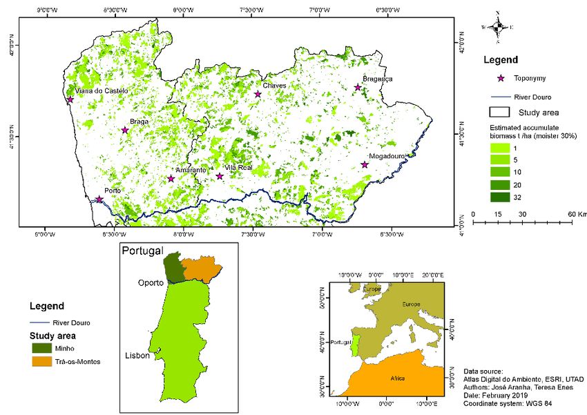
Life 2020, 10, 33                                                                                     2 of 12

occurrence, due to the Mediterranean climate’s influence, the wildfires had a significant impact on
short- and long-term land cover and use. According to the results of the Portuguese National Forest
Inventory (NFI6) [5], in a 15 year time period, from 1995 to 2010, there was a net decrease in Pinus
pinaster forest areas of 263,000 ha (26.6% of the original area), of which 85% was due to its conversion
to the “shrublands and pastures” class of use.
      The increase in wildfire severity in Portugal, reported in recent decades, raises concerns not only
about the long-term adverse effects of fire recurrence in the environment [6,7], but it has also been
demanding attention to this class of land cover. Shrubland areas currently cover more than two million
hectares of the inland Portuguese territory [5]. Additionally, these new shrubland areas constitute the
primary fuel for the frequent wildfires that take place in Portugal.
      On the other hand, shrubs are essential drivers of forest ecosystem productivity and diversity.
Forest understory vegetation is ecologically vital because shrubs, lichens, and mosses can have a
direct effect on belowground processes such as decomposition, nutrient flow, and the accumulation
of soil nutrients [8]. From an environmental point of view, shrublands play an important role,
as they prevent soil erosion and desertification [9], as well as reduce soil erosion more effectively than
trees [10]. They also contribute to soil protection [11], habitat preservation and restoration [12], increase
biodiversity [13], and have a net positive effect on the recruitment of other species [12]. In the long
term, shrub vegetation influences the fluxes of water and sediments by increasing the soil aggregate
stability and cohesion and by improving water infiltration [14].
      Post-fire shrub biomass regrowth evaluation may be, therefore, beneficial for the assessment of
forest services and for calculating the estimates of carbon sequestration and potential energy stock,
while also providing information about the shrub load fuel available, which might be useful for the
prediction of fire behavior [15–18]. The regular harvesting of shrublands might, therefore, additionally
be valuable for diminishing the substantial greenhouse gas emissions associated with these frequent
wildfires [19] through the reduction of forest fire occurrence [20]. Moreover, the increasing interest in
the use of forest biomass for bioenergy production in European countries, as an integrated strategy for
mitigating climate change, increasing renewable energy security, and preventing forest fires, leads to a
reinforced interest in the biomass of the shrubland areas.
      The majority of forestry studies concerning biomass assessment are derived by means of allometric
equations’ calculation, which focus solely on the trees’ biomass estimation. As stated by [21], although
the tree biomass is the principle sink of carbon sequestration in forests, it is also necessary to account
for shrub biomass, as these woody plants play an active role in ecosystem productivity.
      A literature review about forest trees biomass and shrub biomass estimation enabled collecting
several allometric equations (Table 1), for Portuguese regions [22,23], as well as for other countries
(e.g., Central Greece [24] or Southern Spain [25]), were shrubs have different growth rates. The works
in [22] to [25] studied and described the biomass accumulation for the main species occurring in these
areas (e.g., species like Cistus, Erica, Genista, and Ulex; see Table 1). One of these previously presented
equations [23] has the particularity of being able to estimate regenerated shrub biomass of former burnt
areas up to 10 years post-fire. The authors surveyed 45 former burnt areas and adjusted an allometric
equation (see Equation (10)), which can be used in association with a Geographical Information System
project and estimate accumulated biomass in mapped burnt areas. Given that, in the last 30 years of
forest fires in Portugal, fire recurrence ranged from 10 to 15 years [26–30]. The prediction of periods
greater than 10 years is still required.
Life 2020, 10, 33 3 of 12
Table 1. Allometric equations for shrub biomass estimation presented by different authors (bs —shrub
biomass in kg shrub−1 ; Bs —generic shrub biomass in Mg ha−1 ; Bsc —shrub canopy biomass in g m−2 ;
hs —total height of the shrubs (cm); hc —tree canopy height (m); t—time after last fire; CD—shrub
canopy closure (%); h—total height of the tree (m)); and sp. is the abbreviation used for singular species.
Equation Number Allometric Model (Shrub Species) Reference
(1) Bsc = 9.43 − 184.11 t + 1034.2 (Erica sp.)
t2
(2) Bsc = 27.54 t1.202 (Cistus ladanifer L. and Erica sp.)
(3) Bsc = 0.064 t2 + 79.39 t − 76.42 (Cistus ladanifer L.)
[25]
(4) Bsc = 1.58 t2.0714 (Genista and Ulex)
(5) Bsc = 28.06 t1.3868 (Mancha)
(6) Bsc = 1.58 e0.088 t (Pistacia lentiscus L.)
(7) bs = 0.1239 h1.1091
(8) bs = 6.2667(ln t)2.040 [22]
(9) bs = 0.0258 (CDhs )0.754
(10) Bs = 2.002 − 1.211 t + 0.553 t2 − 0.0241 t3
(11) Bs = exp (−1.298 + 1.861 ln t + 0.1265 ln h) [23]
(12) Bs = exp (2.070 + 0.504 ln t + 0.057 ln hs + ln Bsc )
(13) bs = 5.6680 + 0.00008 (hs CD)2
(14) bS = 37.634 + 1.010 t [24]
(15) bs = 5.005 + 0.136 t
The main aim of the authors with the present paper was twofold. First, the study aimed to deepen
the research about biomass assessment for shrubland cover class, supported by different databases in
a Geographic Information System (GIS) project. Secondly, the authors aimed to develop a biomass
model, which could extend the biomass predictions of shrubland cover using GIS, up to the age of 15
years, to embrace the maximum fire recurrence ranges registered in the country.
2. Materials and Methods
2.1. Study area Characteristics
The study area was comprised of 1.9 million ha (Figure 1) located in North Portugal. Although it
was a relatively small region, there were edaphoclimatic and morphological asymmetries (Minho and
Trás-os-Montes regions), as the altitude ranged from sea level (0 m) up to 1410 m in some mountains.
With regard to soils, the origin, type, and characteristics varied greatly depending on the geographical
area. The predominant soil types were Cambisols of both eruptive rocks and shales.
In flat areas crossed by rivers and streams, Fluvisol and Histosol areas were frequent, these areas
being used for agricultural proposes.
In mountainous areas, the predominant soil types were: Rankers, Lithosols, and Luvisols. In some
former burnt areas, where vegetation was reduced to scattered shrubs, bed rock was visible.
The Minho region is located in the NW of Portugal and borders Galicia (Spain) in the north and
the Atlantic Ocean. This region is characterized as having an Atlantic wet climate, with relatively high
exposure to Atlantic Ocean winds, high annual precipitation (1000–2400 mm), and mild summers
(summer mean temperatures from 18 to 22 ◦ C) [31].
Trás-os-Montes is located in the northeastern corner of the country. This region is characterized as
having sub-continental prevailing climate conditions with long cold winters and short, but very hot
and dry summers. The average annual rainfall ranges from 600 up to 1200 mm, and the annual mean
air temperature is 10–14 ◦ C.Life 2020, 10, x FOR PEER REVIEW 4 of 12
Life 2020, 10, 33 4 of 12
Figure 1. Distribution of sampling plots in the study area (North Portugal) and Portugal’s world
Figure geographical location.
1. Distribution of sampling plots in the study area (North Portugal) and Portugal’s world
geographical location.
2.2. Data Sources
This study was supported by 161 sampling plots installed in former burnt areas, within North
2.2. Data Sources
Portugal, in the Minho and Trás-os-Montes regions (Figure 1), for shrub biomass classification
This study was supported by 161 sampling plots installed in former burnt areas, within North
and quantification.
Portugal, in the Minho and Trás-os-Montes regions (Figure 1), for shrub biomass classification and
In the first stage, a Geographic Information System (GIS) project was created using ArcGIS for
quantification.
Desktop (ESRI), in order to map former burnt areas from 1990 up to 2015, made available by the
In the first stage, a Geographic Information System (GIS) project was created using ArcGIS for
Institute of Nature Conservation and Forest (ICNF) and also by the European Forest Fire Information
Desktop (ESRI), in order to map former burnt areas from 1990 up to 2015, made available by the
System (EFFIS). Then, all burnt areas polygons were isolated by burnt time (e.g., 1990, 1991, . . . , 2017)
Institute of Nature Conservation and Forest (ICNF) and also by the European Forest Fire Information
and submitted to a union routine in order to create a new topology for burnt areas’ combination and to
System (EFFIS). Then, all burnt areas polygons were isolated by burnt time (e.g., 1990, 1991, …, 2017)
enable fire recurrence calculation and post-fire time calculation.
and submitted to a union routine in order to create a new topology for burnt areas’ combination and
In the second stage, this information was cross-referenced to CORINE Land Cover maps for 1990,
to enable fire recurrence calculation and post-fire time calculation.
2006, and 2012 (CLC1990, CLC2006, and CLC2012, Copernicus 2018) and Portuguese Land Cover Maps
In the second stage, this information was cross-referenced to CORINE Land Cover maps for
COS 2010 in order to select only burnt areas where pre-fire land cover was shrublands or degraded
1990, 2006, and 2012 (CLC1990, CLC2006, and CLC2012, Copernicus 2018) and Portuguese Land
forest lands.
Cover Maps COS 2010 in order to select only burnt areas where pre-fire land cover was shrublands
The third stage was dedicated to a dynamic table creation that enabled classifying burnt areas
or degraded forest lands.
previously selected according to fire recurrence, last fire occurrence date, and time spent after the fire.
The third stage was dedicated to a dynamic table creation that enabled classifying burnt areas
Then, 10 former burnt areas were selected per each year over the last fire occurrence.
previously selected according to fire recurrence, last fire occurrence date, and time spent after the
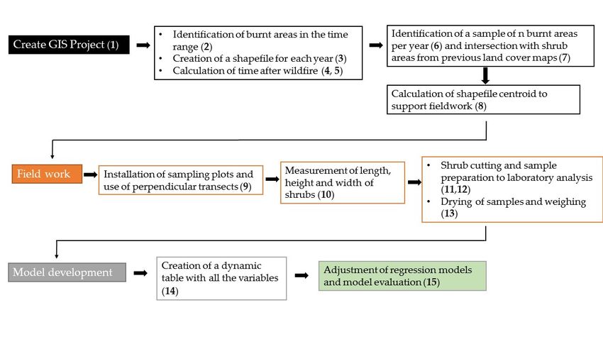
The list of the steps is as follows:
fire. Then, 10 former burnt areas were selected per each year over the last fire occurrence.
1. Create a GIS project to manage burnt areas in inland Portugal.
The list of the steps is as follows:
2. Download burnt area limits shapefiles from 1990 up to 2016.
1. Create a GIS project to manage burnt areas in inland Portugal.
3. Create an independent shapefile for each year.
2. Download burnt area limits shapefiles from 1990 up to 2016.
4. Perform a union routine in order to calculate fire recurrence and the year of the last occurrence.
3. Create an independent shapefile for each year.
5. Calculate the time elapsed since the last occurrence.
4. Perform a union routine in order to calculate fire recurrence and the year of the last occurrence.
6. Identify 10 burnt scars per year after the last occurrence and for the past 15 years, throughout
5. Calculate the time elapsed since the last occurrence.
North Portugal.
6. Identify 10 burnt scars per year after the last occurrence and for the past 15 years, throughout
7. Intersect the burnt areas’ shapefiles to land cover shapefiles in order to isolate only burnt
North Portugal.
patches in shrub areas.
7. Intersect the burnt areas’ shapefiles to land cover shapefiles in order to isolate only burnt
8. Calculate the shapefiles’ centroid point in order to create a sampling network to support field
patches in shrub areas.
work for biophysical data collection.Life 2020, 10, x FOR PEER REVIEW 5 of 12
8. Calculate the shapefiles’ centroid point in order to create a sampling network to support field
Life 2020, 10, 33 5 of 12
work for biophysical data collection.
9. Perform field work for biophysical data collection by means of two perpendicular profile
installations across each
9. Perform field500
work m2 circular plot installed
for biophysical in each sampling
data collection by means plot.
of two perpendicular profile
10. Measureacross
installations the 3each 500 m2 circular
dimensions related plot
to shrubs within
installed thesampling
in each samplingplot.plot: length, width, and
height along each of the
10. Measure the two perpendicular
3 dimensions profiles.
related These
to shrubs values
within theenable
samplingestimating shrub width,
plot: length, densityand
within
heightthe along
sampling eachplot.
of the two perpendicular profiles. These values enable estimating shrub density
11. Cut
within thethe bush and
sampling shrubs at the base and weigh them with a field scale.
plot.
12. Collect
11. Cut shrub
the bush samples (trunk,atbranches,
and shrubs the base and and weigh
leaves)them
to bring
withtoa the
fieldlaboratory.
scale.
13. 12.
DryCollect
the samples, in an open
shrub samples space
(trunk, until 30%
branches, andmoisture
leaves) toand weigh
bring to thethem with a laboratory
laboratory.
scale. 13. Dry the samples, in an open space until 30% moisture and weigh them with a laboratory scale.
14. 14.
Create an Excel
Create an Exceltable using
table the the
using variables: timetime
variables: elapsed since
elapsed the the
since lastlast
fire fire
occurrence, shrub
occurrence, shrub
density
density(percentage
(percentage of land cover
of land estimated
cover estimated during field
during work),
field wetwet
work), weight,
weight,andand
drydryweight.
weight.
15. Adjust
15. Adjustthe regression
the regression models
modelsin order to create
in order an allometric
to create an allometricequation
equationsuitable to be
suitable toused for for
be used
shrub
shrubweight
weightestimation
estimationaccording to the
according time
to the elapsed
time since
elapsed thethe
since lastlast
firefire
occurrence.
occurrence.
Figure
Figure2 shows
2 showsthe the
diagram
diagramof the steps
of the described.
steps described.
Figure 2. Graphic summary of the methodological steps followed in the study.
2.3. Sampling Plots2. Graphic summary of the methodological steps followed in the study.
Figure
In the Minho region, a total of 102 sampling plots were established and surveyed, while in the
2.3. Sampling Plots
region of Trás-os-Montes, 59 plots were established and surveyed, based on former burnt areas’ location.
Only plots
In the withregion,
Minho recurrence
a totalgreater
of 102than or equal
sampling to 2were
plots wereestablished
visited to minimize the possibility
and surveyed, while in the of the
natural
region regeneration of trees
of Trás-os-Montes, Pinusestablished
(e.g.,were
59 plots pinaster, Eucalyptus globulus).
and surveyed, based on former burnt areas’
location.The
Only temporary
plots with plots were of agreater
recurrence circularthan
shape with an
or equal toarea of 500
2 were m2 . In
visited to each plot, two
minimize perpendicular
the possibility
lines
of the (transects)
natural crossingofthe
regeneration center
trees (e.g.,were
Pinus drawn, forEucalyptus
pinaster, shrub canopy density estimation and biometric
globulus).
measurements,
The temporarysuch plotsas shrub
were of length, width,shape
a circular and height.
with an Then,
areaa selection
of 500 mof 2. plants
In each was cut two
plot, off and
weighed in lines
perpendicular the field in ordercrossing
(transects) to obtain thethe greenwere
center weight of the
drawn, forsampled speciesdensity
shrub canopy (Erica sp., Cytisus sp.,
estimation
andChamaespartium tridentatum,such
biometric measurements, andas Ulex
shrubsp.)length,
and towidth,
determine the biomass.
and height. Then, a selection of plants was
After
cut off and the field
weighed inmeasurements
the field in orderwere tocompleted,
obtain the samples of each
green weight ofshrub species species
the sampled were stored
(Ericainsp.,
plastic
bags,sp.,
Cytisus brought to the Forestry
Chamaespartium Sciences
tridentatum, andand Landscape
Ulex sp.) and toArchitecture
determine the of University
biomass. of Trás-os-Montes
and Alto
After theDouro
field (UTAD)
measurementslaboratorywereforcompleted,
further measurements.
samples of eachThese samples
shrub werewere
species then stored
placed in in an
ovenbags, ◦
at 70brought
C in order to be dried out to 30%and moisture. The results achieved, from field and laboratory
plastic to the Forestry Sciences Landscape Architecture of University of Trás-os-
measurements,
Montes and Alto Douro were then(UTAD)used laboratory
to update the forGIS project
further database.
measurements. These samples were then
placed inFrom
an oventhis at
entire
70 °Cdatabase,
in order to 150beplots
dried(ten
outper yearmoisture.
to 30% elapsed after fire occurrence)
The results achieved, were
from selected
field
andinlaboratory
order to be submitted towere
measurements, regression
then usedanalysis and allometric
to update equations’
the GIS project database.adjustment for biomass
calculation. The potential set of regressors referred to the variable time elapsed after the fire (age) and,Life 2020, 10, 33 6 of 12
additionally, to the variables slope, aspect, and altitude, easily obtained from a Digital Elevation Model
(DEM).
3. Results
3.1. Shrubland Characterization
Results (Table 2 and Figure 3) showed that after one year post-fire, the soil was rarely covered by
vegetation and the average biomass weight was around 0.12 Mg ha−1 . Five years after fire occurrence,
the ecosystem was able to regenerate a green canopy that covered near 80% of the land, and after
15 years of a forest fire, the shrubs’ canopy cover could reach 100% and accumulate around 28.9 Mg ha−1
(30% moister) of vegetal biomass.
Table 2. Average (mean ± standard deviation (sd)) and range values of biomass accumulation (Mg ha−1 )
within 15 years after the fire and the respective percentage of canopy cover in the same time interval.
Past Time after the 30% Moisture Shrub Biomass (Mg ha−1 ) Canopy Cover (%)
Fire (Years) Mean ± sd Min − Max Mean ± sd Min − Max
1 0.119 ± 0.027 0.075 − 0.152 0.05 ± 0.04 0.01 − 0.10
2 0.773 ± 0.357 0.266 − 1.57 0.19 ± 0.04 0.12 − 0.23
3 2.595 ± 0.704 1.519 − 3.569 0.34 ± 0.07 0.24 − 0.44
4 4.247 ± 0.886 2.545 − 5.945 0.38 ± 0.02 0.35 − 0.41
5 6.743 ± 1.573 3.451 − 9.48 0.44 ± 0.01 0.42 − 0.45
6 8.556 ± 2.966 3.175 − 12.033 0.48 ± 0.02 0.46 − 0.50
7 9.586 ± 2.397 5.829 − 13.943 0.56 ± 0.02 0.54 − 0.59
8 13.783 ± 3.243 8.124 − 19.126 0.70 ± 0.06 0.64 − 0.77
9 15.368 ± 4.67 5.464 − 21.407 0.81 ± 0.04 0.77 − 0.87
10 19.368 ± 3.282 12.889 − 25.341 0.95 ± 0.03 0.92 − 1.00
11 21.183 ± 3.288 16.271 − 28.656 0.90 ± 0.1 0.80 − 1.00
12 25.285 ± 4.108 14.645 − 30.818 0.98 ± 0.04 0.90 − 1.00
13 25.544 ± 4.089 18.091 − 32.129 0.69 ± 0.17 0.60 − 100
14 26.871 ± 4.763 19.089 − 34.475 0.66 ± 0.23 0.50 − 1.00
Life 2020, 10, x FOR PEER REVIEW 7 of 12
15 28,877 ± 4.427 22.265 − 37596 0.78 ± 0.23 0.50 − 1.00
4.0
Biomass (Mg ha -1)
30% Moisture Shrub biomass
3.5
30% Moisture Shrub biomass average
3.0
2.5
2.0
1.5
1.0
0.5
0.0
0 1 2 3 4 5 6 7 8 9 10 11 12 13 14 15 16
Time after wildfire (years)
Figure 3. Accumulated biomass evolution over 15 years after fire and adjustment of the accumulated
Figure 3. Accumulated biomass evolution over 15 years after fire and adjustment of the accumulated
average amounts to Equation (16).
average amounts to Equation (16).
In the case of a polynomial model, the presence of multicollinearity was expected, and the
statistical analysis carried out through the factors of inflation of the variance confirmed the existence
of this. However, this phenomenon could only represent a problem when the model is applied to
new data different from those that were used in the estimation of the model, which was not the case,
due to the convenience of using regional models [32,33]. It should be advisable, therefore, to evaluate
its performance (and proceed with adjustment of the values of the estimated parameters, if needed),Life 2020, 10, 33 7 of 12
3.2. Allometric Model for Shrub Biomass Estimation
In the first stage, post-fire age (t) and shrub biomass (B) variables were depicted in a bivariate
plot to analyze the relationship type that could be established between age and biomass. The graphic
representation showed a sigmoidal distribution, which led to the use of a non-linear approach.
In the second stage, several linear and non-linear regression models were adjusted by means of
the Method of Least Squares (MLS) using JMP software and ranked according to the higher adjusted
determination coefficient (R2adj ) and lower Root Mean Squared Error (RMSE). From the potential
set of regressors, “time post-fire” was retained as a significant explanatory variable. A third-degree
polynomial model (Y = β0 + β1 X + β2 X2 + β3 X3 + ε) was selected as a proper model for the description
of the relationship between B and t:
B = −0.0461 − 0.0398t + 0.3122t2 − 0.0121t3 (16)
R2adj = 0.8978, RMSE = 3.31 Mg ha−1 , n = 150 observations, p-value < 0.01.
where B is the shrub biomass (Mg ha−1 at 30% moister) and t is the time post-fire (years).
In the case of a polynomial model, the presence of multicollinearity was expected, and the
statistical analysis carried out through the factors of inflation of the variance confirmed the existence
of this. However, this phenomenon could only represent a problem when the model is applied to
new data different from those that were used in the estimation of the model, which was not the case,
due to the convenience of using regional models [32,33]. It should be advisable, therefore, to evaluate
its performance (and proceed with adjustment of the values of the estimated parameters, if needed),
before considering the use of the proposed model (Equation (16)) in different regions.
4. Discussion
4.1. Shrubland Characterization
In general, shrub canopy cover percentage varied according to shrub species present. If Cytisus sp.
was the dominant species, five years after the fire, they reached 100% occupancy. In high mountain
areas, where the dominant shrubs were mainly Erica sp. and Chamaespartium tridentatum, the coverage
percentage hardly reached 100% (above an 800 m altitude, coverage rarely reached 100%). Altitude
seemed to be a leading variable that controlled shrub canopy land cover. The higher the land, the lower
the canopy density.
4.2. Allometric Model for Shrub Biomass Estimation
This research was driven by the need to adjust a new allometric equation to estimate regenerated
shrub biomass since previously presented models (Viana et al. [22], Equation (8), and Aranha et al. [23],
Equation (10)) were not accurate to be applied to the entire study area or for extended time periods.
The new calculated model was compared to the previous ones in order to demonstrate its fitting
adequacy, as presented in Figure 4.Life 2020, 10, 33 8 of 12
Life 2020, 10, x FOR PEER REVIEW 8 of 12
Viana et al. [22]
60
Biomass (Mg ha-1)
55
Aranha et al. [23]
50
45
40
New model
35
30 30% Moisture Shrub
25 biomass average
20
15
10
5
0
0 1 2 3 4 5 6 7 8 9 10 11 12 13 14 15 16 17 18
Time after Wildfire (years)
Figure4.4. Graphic
Figure representation of
Graphic representation of biomass
biomassaccumulated
accumulatedafter
afterwildfire
wildfireduring
during1717years
yearsaccording
according
to
to [22,23], Equations (8) and (10), respectively, and the new model, Equation (16). The black circles are
[22,23], Equations (8) and (10), respectively, and the new model, Equation (16). The black circles are
the average values of shrub biomass (30% of moisture).
the average values of shrub biomass (30% of moisture).
The equation adjusted by [22] was based on information collected from 18 sampling plots for age
The equation adjusted by [22] was based on information collected from 18 sampling plots for
ranging from two to seven years. Thus, the estimates of biomass values for the age over seven years
age ranging from two to seven years. Thus, the estimates of biomass values for the age over seven
were extrapolations. The equation adjusted by [23] was based on information from 45 sampling plots,
years were extrapolations. The equation adjusted by [23] was based on information from 45 sampling
with time elapsed post-fire from two to 10 years, which allowed estimating biomass values up to 14
plots, with time elapsed post-fire from two to 10 years, which allowed estimating biomass values up
years. After this age, the model originated decreasing values, as can be seen in the curve inflection
to 14 years. After this age, the model originated decreasing values, as can be seen in the curve
depicted in Figure 4. The new model presented in this study was adjusted to data from 150 sampling
inflection depicted in Figure 4. The new model presented in this study was adjusted to data from 150
plots and allowed reasonable extrapolations between 15 and 17 years. In the specific case of forest fires
sampling plots and allowed reasonable extrapolations between 15 and 17 years. In the specific case
in Portugal, which have fire cycles of 10 to 15 years, this new equation allowed estimating biomass
of forest fires in Portugal, which have fire cycles of 10 to 15 years, this new equation allowed
accumulation after fire for that period. It is worthwhile mentioning that shrublands are systems
estimating biomass accumulation after fire for that period. It is worthwhile mentioning that
that are not usually managed, nor particularly disturbed. As age increases, the same happens with
shrublands are systems that are not usually managed, nor particularly disturbed. As age increases,
their biomass accumulation. The large dataset used in this study allowed evidencing this trend (with
the same happens with their biomass accumulation. The large dataset used in this study allowed
the proportion of variance explained of nearly 0.90). Since all this research was derived using GIS
evidencing this trend (with the proportion of variance explained of nearly 0.90). Since all this
techniques, the model could be assigned to burnt area maps and depicted as spatial biomass maps,
research was derived using GIS techniques, the model could be assigned to burnt area maps and
as shown in Figure 5.
depicted as spatial biomass maps, as shown in Figure 5.
Using GIS facilities and making burnt area times post-fire accumulated biomass a function of the
Using GIS facilities and making burnt area times post-fire accumulated biomass a function of
time elapsed after the fire, it could be verified that in the north of Portugal, the total accumulated
the time elapsed after the fire, it could be verified that in the north of Portugal, the total accumulated
biomass was 4,947,428 Mg in former burnt areas.
biomass was 4,947,428 Mg in former burnt areas.
The installation of a large number of sampling plots and fieldwork for data collection and
The installation of a large number of sampling plots and fieldwork for data collection and
measurement are time consuming and costly, which, in large areas, may limit the studies’ feasibility.
measurement are time consuming and costly, which, in large areas, may limit the studies’ feasibility.
Therefore, the use of expeditious and low-cost techniques, such as the use of allometric equations to
Therefore, the use of expeditious and low-cost techniques, such as the use of allometric equations to
quantify shrub biomass, is a good alternative for estimating plant biomass.
quantify shrub biomass, is a good alternative for estimating plant biomass.
Although altitude was identified as a variable that controlled shrub canopy land cover, the time
Although altitude was identified as a variable that controlled shrub canopy land cover, the time
elapsed after a fire was identified as the variable with a major impact on the assessment of shrub biomass.
elapsed after a fire was identified as the variable with a major impact on the assessment of shrub
It is worthwhile mentioning that there are no barriers related to GIS utilization in shrub biomass
biomass.
location and calculation tasks, as evidenced by the numerous articles written on the subject, e.g., [34–40].
The major constraints to the shrubs’ biomass use after GIS calculation are related to the costs of cutting,
removing, and transporting biomass from the forest areas to the places of use. The amount paid for
biomass does not offset the cost of exploration. Previous published results, e.g., [34], recommended a
maximum distance of 35 km from biomass harvesting places to power plants. Today, due to the price
of fuel, tolls, and minimum wage, the maximum distance for exploration and transportation is reducedLife 2020, 10, 33 9 of 12
Life 2020, 10, x FOR PEER REVIEW 9 of 12
to less than half (15 km). It is not for lack of information (satellite images and geo-referenced data) that
the forest accumulates in the forests, but it is for the lack of policies to enhance biomass value as a
raw material.
Figure 5. Spatial distribution of the amount of biomass accumulated in burned areas in the north of
Figure 5. Spatial distribution of the amount of biomass accumulated in burned areas in the north of
Portugal, during 27 years
Portugal, during (1990–2017), expressed
27 years (1990–2017), in Mg
expressed ha−1.
in Mg ha−1 .
5. Conclusions
It is worthwhile mentioning that there are no barriers related to GIS utilization in shrub biomass
The achieved
location and calculation results
tasks, as enable statingby
evidenced that thenumerous
the woody shrub species,written
articles which areon regenerated aftere.g.,
the subject, the [34–
fires, reach high values of biomass in a few years. These results point to the remarkable ecological
40]. The major constraints to the shrubs’ biomass use after GIS calculation are related to the costs of
dynamics of this stratum and potential interest for commercial purposes.
cutting, removing, The and transporting
allometric biomass was
equation presented fromsuitable
the forest
to applyareas to the burnt
to former places of use.
areas The
within amount
North
paid for biomass
Portugal,does not offset
with post-fire the cost
ages ranging fromofoneexploration.
to 17 years, to Previous published
predict the amount results, shrub
of accumulated e.g., [34],
recommended a maximum
biomass distance ofmethods,
using non-destructive 35 km from givenbiomass harvesting
the time elapsed places
after the fire. to power plants. Today,
When used with remote sensing or GIS techniques,
due to the price of fuel, tolls, and minimum wage, the maximum distance it allows creating mapsfor
of shrub biomass and
exploration
accumulated in former burnt areas and to analyze its spatial distribution. This issue is of particular
transportation is reduced to less than half (15 km). It is not for lack of information (satellite images
importance because it will enable locating where there is more accumulated biomass. In this way, it is
and geo-referenced
possible todata)
knowthat thethe
where forest accumulates
fire hazard is higher in
andthe
to forests, but itattention
pay particular is for the lack of
to these policies
places in to
enhance biomass valueactions
surveillance as a raw
or to material.
identify where biomass can be harvested for energy purposes. In both cases,
the procedures will protect the forested land. It can be highlighted that the methodology presented in
5. Conclusions
this study can be straightforwardly replicated in other regions.
Author Contributions:
The achieved results enable Conceptualization,
stating thatJ.A.; theperformed
woodythe experiment
shrub and analysis,
species, whichJ.A.,
areT.E., T.F., and J.L.; after
regenerated
performed the statistical analysis, J.A., T.E., T.F., and J.L.; resources, H.V., A.C., and J.A.; writing, original draft
the fires, reach high values
preparation, T.E. andof biomass
J.A.; in a few
writing, review years. J.A.,
and editing, These T.F., results pointadministration,
and J.L.; project to the remarkable ecological
J.A. All authors
read and agreed to the published version of the manuscript.
dynamics of this stratum and potential interest for commercial purposes.
Funding: This research was funded by the INTERACT project “Integrated Research in Environment, Agro-Chain
The allometric equation presented was suitable to apply to former burnt areas within North
and Technology”, No. NORTE-01-0145-FEDER-000017, in its line of research entitled BEST, co-financed
Portugal, with post-fire
by the Europeanages ranging
Regional from Fund
Development one (ERDF)
to 17 years,
through to predict
NORTE 2020the amount
(North RegionalofOperational
accumulated
Program 2014/2020). For authors integrated in the CITAB research center, it was further financed by the
shrub biomass using non-destructive methods,
FEDER/COMPETE/POCI-Operational given the
Competitiveness andtime elapsed afterProgramme,
Internationalization the fire. under Project
POCI-01-0145-FEDER-006958, and by National Funds by FCT
When used with remote sensing or GIS techniques, it allows creating maps of (the Portuguese Foundation for shrub
Science biomass
and
accumulated in former burnt areas and to analyze its spatial distribution. This issue is of particular
importance because it will enable locating where there is more accumulated biomass. In this way, it
is possible to know where the fire hazard is higher and to pay particular attention to these places in
surveillance actions or to identify where biomass can be harvested for energy purposes. In both cases,Life 2020, 10, 33 10 of 12
Technology), under the project UID/AGR/04033/2020. The participation of the co-author Teresa Fonseca was
financed by National Funds through the Portuguese funding agency, FCT, within project UIDB/00239/2020.
Conflicts of Interest: The authors declare no conflict of interest.
References
1. Caetano, M.; Igreja, C.; Marcelino, F.; Costa, H. Estatísticas e dinâmicas territoriais multiescala de Portugal
Continental 1995-2007-2010 com base na Carta de Uso e Ocupação do Solo (COS). Direcção Geral Territ. 2017,
149.
2. Serra, P.; Pons, X.; Saurí, D. Land-cover and land-use change in a Mediterranean landscape: A spatial analysis
of driving forces integrating biophysical and human factors. Appl. Geogr. 2008, 28, 189–209. [CrossRef]
3. Mateus, P.; Fernandes, P.M.P. The Portuguese Forest Based Chains: Sector Analyses. In Forest Context
and Policies in Portugal, Present and Future Challenges, World Forests; Reboredo, F., Ed.; Springer: Cham,
Switzerland, 2014; Volume 19, ISBN 9783319084541.
4. Ursino, N.; Romano, N. Wild forest fire regime following land abandonment in the Mediterranean region.
Geophys. Res. Lett. 2014, 41, 8359–8368. [CrossRef]
5. ICNF. I F N 6—Áreas dos Usos do Solo e das Espécies Florestais de Portugal Continental 1995-2005-2010;
Preliminary Report. 2013. Available online: http://www2.icnf.pt/portal/florestas/ifn/resource/ficheiros/ifn/
ifn6-res-prelimv1-1 (accessed on 27 March 2019).
6. Hosseini, M.; Geissen, V.; González-Pelayo, O.; Serpa, D.; Machado, A.I.; Ritsema, C.; Keizer, J.J. Effects of fire
occurrence and recurrence on nitrogen and phosphorus losses by overland flow in maritime pine plantations
in north-central Portugal. Geoderma 2017, 289, 97–106. [CrossRef]
7. Bento-Gonçalves, A.J.; Vieira, A.V.; Costa, M.R.M. Perspectives, Issues and Challenges of the 21st Century; Nova
Science Publishers: Hauppauge, NY, USA, 2018.
8. Huff, S.; Poudel, K.P.; Ritchie, M.; Temesgen, H. Quantifying aboveground biomass for common shrubs
in northeastern California using nonlinear mixed effect models. Forest Ecol. Manag. 2018, 424, 154–163.
[CrossRef]
9. Imeson, A. Desertification, Land Degradation and Sustainability; John Wiley & Sons: West Sussex, UK, 2012;
ISBN 1119978483.
10. Cerdá, A.; Doerr, S.H. Influence of vegetation recovery on soil hydrology and erodibility following fire:
An 11-year investigation. Int. J. Wildland Fire 2005, 14, 423–437. [CrossRef]
11. Bochet, E.; Poesen, J.; Rubio, J.L. Runoff and soil loss under individual plants of a semi-arid Mediterranean
shrubland: Influence of plant morphology and rainfall intensity. Earth Surf. Process. Landf. 2006, 31, 536–549.
[CrossRef]
12. Gómez-Aparicio, L.; Zamora, R.; Gómez, J.M.; Hódar, J.A.; Castro, J.; Baraza, E. Applying plant facilitation
to forest restoration: A meta-analysis of the use of shrubs as nurse plants. Ecol. Appl. 2004, 14, 1128–1138.
[CrossRef]
13. Mangas, J.G.; Lozano, J.; Cabezas-Díaz, S.; Virgós, E. The priority value of scrubland habitats for carnivore
conservation in Mediterranean ecosystems. Biodivers. Conserv. 2008, 17, 43–51. [CrossRef]
14. Zuazo, V.H.D.; Pleguezuelo, C.R.R. Soil-erosion and runoff prevention by plant covers. A review. Agron.
Sustain. Dev. 2008, 28, 65–86. [CrossRef]
15. Botelho, S.; Vegao, J.A.; Fernandescl, P.; Rego, F.M.C. Prescribed Fire Behavior and Fuel Consumption in
Northern Portugal and Galiza Maritime Pine Stands. In Proceedings of the 2nd international Conference
Forest Fire Research, Coimbra, Portugal, 21–24 November 1994.
16. Rego, F.C.; Pereira, J.P.; Fernandes, P.M.; Almeida, A.F. Biomass and Aerial Structure Characteristics of Some
Mediterranean Shrub Species. In Proceedings of the 2nd International Conference on Forest Fire Research B,
Coimbra, Portugal, 21–24 November 1994; pp. 377–384.
17. Fernandes, P.M.; Rego, F.C. Equations for Fuel Loading Estimation in Shrub Communities Dominated by
Chamaespartium Tidentatum and Erica Umbellata. In Proceedings of the III International Conference on
Forest Fire Research, Luso, Portugal, 16–20 November 1998; pp. 2553–2564.Life 2020, 10, 33 11 of 12
18. Molina, J.R.; García, J.P.; Fernández, J.J.; Rodríguez y Silva, F. Prescribed fire experiences on crop residue
removal for biomass exploitations. Application to the maritime pine forests in the Mediterranean Basin.
Sci. Total Environ. 2018, 612, 63–70. [CrossRef] [PubMed]
19. Silva, T.P.; Pereira, J.M.; Paúl, J.C.; Santos, M.T.; Vasconcelos, M.J. Estimativa de Emissões Atmosféricas
Originadas por Fogos Rurais em Portugal Estimate of Atmospheric Emissions Originated by Wildfires in
Portugal. Silva Lusit. 2006, 14, 239–263.
20. Viana, H. Modelling and Mapping Aboveground Biomass for energy Usage and Carbon Storage Assessment
in Mediterranean Ecosystems. Ph.D. Thesis, Universidade de Trás os Montes e Alto Douro, Vila Real,
Portugal, 2012.
21. Cairns, M.A.; Lajtha, K.; Beedlow, P.A. Dissolved carbon and nitrogen losses from forests of the Oregon
Cascades over a successional gradient. Plant Soil 2009, 318, 185–196. [CrossRef]
22. Viana, H.; Fernandes, P.; Rocha, R.; Lopes, D.; Aranha, J. Alometria, Dinâmicas da Biomassa e do Carbono
Fixado em Algumas Espécies Arbustivas de Portugal. In Proceedings of the 6º Congresso Florestal Nacional,
Ponta Delgada, Portugal, 6–9 October 2009; pp. 244–252.
23. Aranha, J.; Calvão, A.R.; Lopes, D.; Viana, H. Quantificação Da Biomassa Consumida Nos Últimos 20 Anos
De Fogos Florestais No Norte Portugal. Rev. İnf. Ordem Eng. REGIÃO NORTE 2011, Info26, 44–49.
24. Kazanis, D.; Xanthopoulos, G.; Arianoutsou, M. Understorey fuel load estimation along two post-fire
chronosequences of Pinus halepensis Mill. forests in Central Greece. J. Forest Res. 2012, 17, 105–109.
[CrossRef]
25. Navarro Cerrillo, R.M.; Oyonarte, P.B. Estimation of above-ground biomass in shrubland ecosystems of
southern Spain. Forest Syst. 2006, 15, 197–207. [CrossRef]
26. Moreira, F.; Rego, F.C.; Ferreira, P.G. Temporal (1958–1995) pattern of change in a cultural landscape of
northwestern Portugal: Implications for fire occurrence. Landsc. Ecol. 2001, 16, 557–567. [CrossRef]
27. Ferreira Leite, F.; Bento Gonçalves, A.; Vieira, A. The recurrence interval of forest fires in Cabeço da Vaca
(Cabreira Mountain-northwest of Portugal). Environ. Res. 2011, 111, 215–221. [CrossRef]
28. Oliveira, S.L.J.; Pereira, J.M.C.; Carreiras, J.M.B. Fire frequency analysis in Portugal (1975–2005), using
Landsat-based burnt area maps. Int. J. Wildland Fire 2011, 21, 48–60. [CrossRef]
29. Pereira, M.G.; Aranha, J.; Amraoui, M. Land cover fire proneness in Europe. Forest Syst. 2014, 23, 598–610.
[CrossRef]
30. Fernandes, P.M.; Fernandes, M.M.; Loureiro, C. Post-fire live residuals of maritime pine plantations in
Portugal: Structure, burn severity, and fire recurrence. Forest Ecol. Manag. 2015, 347, 170–179. [CrossRef]
31. Moreno, J.; Fatela, F.; Moreno, F.; Leorri, E.; Taborda, R.; Trigo, R. Grape harvest dates as indicator of
spring-summer mean maxima temperature variations in the Minho region (NW of Portugal) since the 19th
century. Glob. Planet. Chang. 2016, 141, 39–53. [CrossRef]
32. Alin, A. Multicollinearity. Wiley Interdiscip. Rev. Comput. Stat. 2010, 2, 370–374. [CrossRef]
33. Dormann, C.F.; Elith, J.; Bacher, S.; Buchmann, C.; Carl, G.; Carré, G.; Marquéz, J.R.G.; Gruber, B.;
Lafourcade, B.; Leitão, P.J.; et al. Collinearity: A review of methods to deal with it and a simulation study
evaluating their performance. Ecography 2013, 36, 27–46. [CrossRef]
34. Viana, H.; Cohen, W.B.; Lopes, D.; Aranha, J. Assessment of forest biomass for use as energy. GIS-based
analysis of geographical availability and locations of wood-fired power plants in Portugal. Appl. Energy
2010, 87, 2551–2560. [CrossRef]
35. Wijaya, A.; Kusnadi, S.; Gloaguen, R.; Heilmeier, H. Improved strategy for estimating stem volume and forest
biomass using moderate resolution remote sensing data and GIS. J. Forest Res. 2010, 21, 1–12. [CrossRef]
36. Deng, S.; Shi, Y.; Jin, Y.; Wang, L. A GIS-based approach for quantifying and mapping carbon sink and stock
values of forest ecosystem: A case study. Energy Procedia 2011, 5, 1535–1545. [CrossRef]
37. Singh, T.P.; Das, S. Predictive Analysis for Vegetation Biomass Assessment in Western Ghat Region (WG)
Using Geospatial Techniques. J. Indian Soc. Remote Sens. 2014, 42, 549–557. [CrossRef]
38. Botequim, B.; Zubizarreta-Gerendiain, A.; Garcia-Gonzalo, J.; Silva, A.; Marques, S.; Fernandes, P.M.;
Pereira, J.M.C.; Tomé, M. A model of shrub biomass accumulation as a tool to support management of
portuguese forests. iForest 2014, 8, 114–125. [CrossRef]Life 2020, 10, 33 12 of 12
39. Nguyen, H.K.; Nguyen, B.N. Mapping biomass and carbon stock of forest by remote sensing and GIS
technology at Bach Ma National Park, Thua Thien Hue province. J. Vietnam Environ. 2016, 8, 80–87.
40. Quinta-Nova, L.; Fernandez, P.; Pedro, N. GIS-Based Suitability Model for Assessment of Forest Biomass
Energy Potential in a Region of Portugal. Earth Environ. Sci. 2017, 95, 042059. [CrossRef]
© 2020 by the authors. Licensee MDPI, Basel, Switzerland. This article is an open access
article distributed under the terms and conditions of the Creative Commons Attribution
(CC BY) license (http://creativecommons.org/licenses/by/4.0/).You can also read