Learning Human Pose Estimation Features with Convolutional Networks
←
→
Page content transcription
If your browser does not render page correctly, please read the page content below
Learning Human Pose Estimation Features with
Convolutional Networks
Arjun Jain Jonathan Tompson Mykhaylo Andriluka
New York University New York University MPI Saarbruecken
ajain@nyu.edu tompson@cims.nyu.edu andriluk@mpi-inf.mpg.de
Graham W. Taylor Christoph Bregler
University of Guelph New York University
gwtaylor@uoguelph.ca chris.bregler@nyu.edu
Abstract
This paper introduces a new architecture for human pose estimation using a multi-
layer convolutional network architecture and a modified learning technique that
learns low-level features and a higher-level weak spatial model. Unconstrained
human pose estimation is one of the hardest problems in computer vision, and our
new architecture and learning schema shows improvement over the current state-
of-the-art. The main contribution of this paper is showing, for the first time, that
a specific variation of deep learning is able to meet the performance, and in many
cases outperform, existing traditional architectures on this task. The paper also
discusses several lessons learned while researching alternatives, most notably, that
it is possible to learn strong low-level feature detectors on regions that might only
cover a few pixels in the image. Higher-level spatial models improve somewhat
the overall result, but to a much lesser extent than expected. Many researchers
previously argued that the kinematic structure and top-down information are cru-
cial for this domain, but with our purely bottom-up, and weak spatial model, we
improve on other more complicated architectures that currently produce the best
results. This echos what many other researchers, like those in the speech recogni-
tion, object recognition, and other domains have experienced [26].
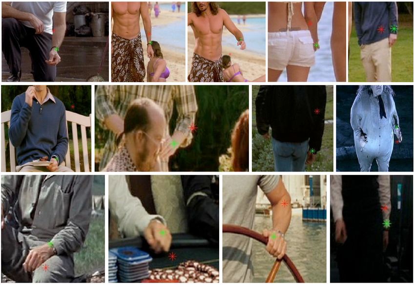
Figure 1: The green cross is our new technique’s wrist locator, the red cross is the state-of-the-art
CVPR13 MODEC detector [38] on the FLIC database.
1 Introduction
One of the hardest tasks in computer vision is determining the high degree-of-freedom configuration
of a human body with all its limbs, complex self-occlusion, self-similar parts, and large variations
due to clothing, body-type, lighting, and many other factors. The most challenging scenario for
this problem is from a monocular RGB image and with no prior assumptions made using motion
models, pose models, background models, or any other common heuristics that current state-of-the-
art systems utilize. Finding a face in frontal or side view is relatively simple, but determining the
1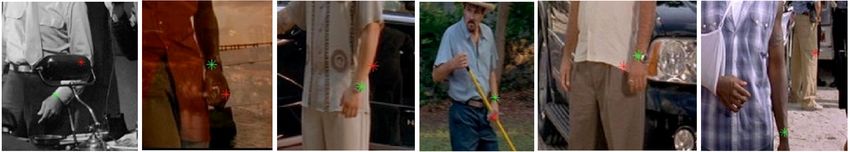
exact location of body parts such as hands, elbows, shoulders, hips, knees and feet, each of which
sometimes only occupy a few pixels in the image in front of an arbitrary cluttered background, is
significantly harder.
The best performing pose estimation methods, including those based on deformable part models,
typically are based on body part detectors. Such body part detectors commonly consist of multiple
stages of processing. The first stage of processing in a typical pipeline consists of extracting sets
of low-level features such as SIFT [25], HoG [11], or other filters that describe orientation statistics
in local image patches. Next, these features are pooled over local spatial regions and sometimes
across multiple scales to reduce the size of the representation and also develop local shift/scale
invariance. Finally, the aggregate features are mapped to a vector, which is then either input to 1)
a standard classifier such as a support vector machine (SVM) or 2) the next stage of processing
(e.g. assembling the parts into a whole). Much work is devoted to engineering the system to produce
a vector representation that is sensitive to class (e.g. head, hands, torso) while remaining invariant
to the various nuisance factors (lighting, viewpoint, scale, etc.)
An alternative approach is representation learning: relying on the data instead of feature engineer-
ing, to learn a good representation that is invariant to nuisance factors. For a recent review, see
[6]. It is common to learn multiple layers of representation, which is referred to as deep learning.
Several such techniques have used unsupervised or semi-supervised learning to extract multi-layer
domain-specific invariant representations, however, it is purely supervised techniques that have won
several recent challenges by large margins, including ImageNet LSVRC 2012 and 2013 [23, 51].
These end-to-end learning systems have capitalized on advances in computing hardware (notably
GPUs), larger datasets like ImageNet, and algorithmic advances (specifically gradient-based train-
ing methods and regularization).
While these methods are now proven in generic object recognition, their use in pose estimation has
been limited. Part of the challenge in making end-to-end learning work for human pose estimation is
related to the nonrigid structure of the body, the necessity for precision (deep recognition systems of-
ten throw away precise location information through pooling), and the complex, multi-modal nature
of pose.
In this paper, we present the first end-to-end learning approach for full-body human pose estima-
tion. While our approach is based on convolutional networks (convnets) [24], we want to stress
that the naı̈ve implementation of applying this model “off-the-shelf” will not work. Therefore, the
contribution of this work is in both a model that outperforms state of the art deformable part models
(DPMs) on a modern, challenging dataset, and also an analysis of what is needed to make convnets
work in human pose estimation. In particular, we present a two-stage filtering approach whereby
the response maps of convnet part detectors are denoised by a second process informed by the part
hierarchy.

2   Related Work

Detecting people and their pose has been investigated for decades. Many early techniques rely
on sliding-window part detectors based on hand-crafted or learned features or silhouette extraction
techniques applied to controlled recording conditions. Examples include [14, 49, 5, 30]. We refer to
[35] for a complete survey of this era. More recently, several new approaches have been proposed
that are applied to unconstrained domains. In such domains, good performance has been achieved
with so-called “bag of features” followed by regression-based, nearest neighbor or SVM-based ar-
chitectures. Examples include “shape-context” edge-based histograms from the human body [28, 1]
or just silhouette features [19]. Shakhnarovich et al. [39] learn a parameter sensitive hash function to
perform example-based pose estimation. Many relevant techniques have also been applied to hand
tracking such as [48]. A more general survey of the large field of hand tracking can be found in [12].
Many techniques have been proposed that extract, learn, or reason over entire body features. Some
use a combination of local detectors and structural reasoning (see [36] for coarse tracking and [10]
for person-dependent tracking). In a similar spirit, more general techniques using pictorial structures
[2, 3, 17, 37, 33, 34], “poselets” [9], and other part-models [16, 50] have received increased attention.
We will focus on these techniques and their latest incarnations in the following sections.

                                                   2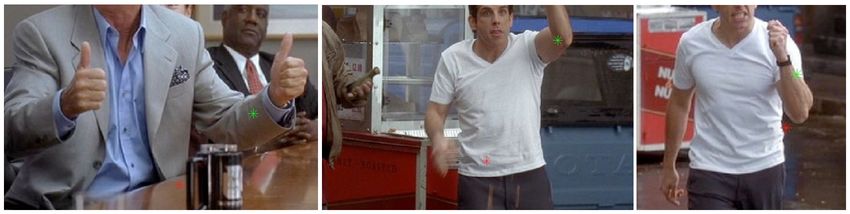
Further examples come from the HumanEva dataset competitions [41], or approaches that use
higher-resolution shape models such as SCAPE [4] and further extensions [20, 8]. These differ
from our domain in that the images considered are of higher quality and less cluttered. Also many
of these techniques work on images from a single camera, but need video sequence input (not single
images) to achieve impressive results [42, 52].
As an example of a technique that works for single images against cluttered backgrounds, Shotton et
al.’s Kinect based body part detector [40] uses a random forest of decision trees trained on synthetic
depth data to create simple body part detectors. In the proposed work, we also adopt simple part-
based detectors, however, we focus on a different learning strategy.
There are a number of successful end-to-end representation learning techniques which perform pose
estimation on a limited subset of body parts or body poses. One of the earliest examples of this type
was Nowlan and Platt’s convolutional neural network hand tracker [30], which tracked a single hand.
Osadchy et al. applied a convolutional network to simultaneously detect and estimate the pitch, yaw
and roll of a face [31]. Taylor et al. [44] trained a convolutional neural network to learn an embedding
in which images of people in similar pose lie nearby. They used a subset of body parts, namely, the
head and hand locations to learn the “gist” of a pose, and resorted to nearest-neighbour matching
rather than explicitly modeling pose. Perhaps most relevant to our work is Taylor et al.’s work on
tracking people in video [45], augmenting a particle filter with a structured prior over human pose
and dynamics based on learning representations. While they estimated a posterior over the whole
body (60 joint angles), their experiments were limited to the HumanEva dataset [41], which was
collected in a controlled laboratory setting. The datasets we consider in our experiments are truly
poses “in the wild”, though we do not consider dynamics.
A factor limiting earlier methods from tacking full pose-estimation with end-to-end learning meth-
ods, in particular deep networks, was the limited amount of labeled data. Such techniques, with
millions or more parameters, require more data than structured techniques that have more a priori
knowledge, such as DPMs. We attack this issue on two fronts. First, directly, by using larger labeled
training sets which have become available in the past year or two, such as FLIC [38]. Second, in-
directly, by better exploiting the data we have. The annotations provided by typical pose estimation
datasets contain much richer information compared to the class labels in object recognition datasets
In particular, we show that the relationships among parts contained in these annotations can be used
to build better detectors.

3   Model

To perform pose estimation with a convolutional network architecture [24] (convnet), the most ob-
vious approach would be to map the image input directly to a vector coding the articulated pose: i.e.
the type of labels found in pose datasets. The convnet output would represent the unbounded 2-D
or 3-D positions of joints, or alternatively a hierarchy of joint angles. However, we found that this
worked very poorly. One issue is that pooling, while useful for improving translation invariance dur-
ing object recognition, destroys precise spatial information which is necessary to accurately predict
pose. Convnets that produce segmentation maps, for example, avoid pooling completely [47, 13].
Another issue is that the direct mapping from input space to kinematic body pose coefficients is
highly non-linear and not one-to-one. However, even if we took this route, there is a deeper issue
with attempting to map directly to a representation of full body pose. Valid poses represent a much
lower-dimensional manifold in the high-dimensional space in which they are captured. It seems
troublesome to make a discriminative network map to a space in which the majority of configura-
tions do not represent valid poses. In other words, it makes sense to restrict the net’s output to a
much smaller class of valid configurations.
Rather than perform multiple-output regression using a single convnet to learn pose coefficients
directly, we found that training multiple convnets to perform independent binary body-part clas-
sification, with one network per feature, resulted in improved performance on our dataset. These
convnets are applied as sliding windows to overlapping regions of the input, and map a window of
pixels to a single binary output: the presence or absence of that body part. The result of applying
the convnet is a response-map indicating the confidence of the body part at that location. This lets
us use much smaller convnets, and retain the advantages of pooling, at the expense of having to
maintain a separate set of parameters for each body part. Of course, a series of independent part

                                                   3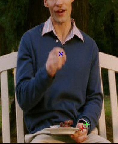
RGB (LCN)             16 feats         32 feats         32 feats         8192
 64x64px              32x32px          16x16px          16x16px                       500
                                                                                                 100
                                                                   reshape                                 1

                     5x5 Conv         5x5 Conv         5x5 Conv                                  Full
                                                                                          Full +logistic
                      +ReLU            +ReLU            +ReLU                 Full       +ReLU
                     +MaxPool         +MaxPool                               +ReLU
               Figure 2: The convolutional network architecture used in our experiments.

detectors cannot enforce consistency in pose in the same way as a structured output model, which
produces valid full-body configurations. In the following sections, we first describe in detail the con-
volutional network architecture and then a method of enforcing pose consistency using parent-child
relationships.

3.1       Convolutional Network Architecture

The lowest level of our two-stage feature detection pipeline is based on a standard convnet architec-
ture, an overview of which is shown in Figure 2. Convnets, like their fully-connected, deep neural
network counterparts, perform end-to-end feature learning and are trained with the back-propagation
algorithm. However, they differ in a number of respects, most notably local connectivity, weight
sharing, and local pooling. The first two properties significantly reduce the number of free parame-
ters, and reduce the need to learn repeated feature detectors at different locations of the input. The
third property makes the learned representation invariant to small translations of the input.
The convnet pipeline shown in Figure 2 starts with a 64×64 pixel RGB input patch which has
been local contrast normalized (LCN) [22] to emphasize geometric discontinuities and improve
generalization performance [32]. The LCN layer is comprised of a 9×9 pixel local subtractive
normalization, followed by a 9×9 local divisive normalization. The input is then processed by three
convolution and subsampling layers, which use rectified linear units (ReLUs) [18] and max-pooling.
As expected, we found that internal pooling layers help to a) reduce computational complexity1 and
b) improve classification tolerance to small input image translations. Unfortunately, pooling also
results in a loss of spatial precision. Since the target application for this convnet was offline (rather
than real-time) body-pose detection, and since we found that with sufficient training exemplars,
invariance to input translations can be learned, we choose to use only 2 stages of 2 × 2 pooling
(where the total image downsampling rate is 4 × 4).
Following the three stages of convolution and subsampling, the top-level pooled map is flattened
to a vector and processed by three fully connected layers, analogous to those used in deep neural
networks. Each of these output stages is composed of a linear matrix-vector multiplication with
learned bias, followed by a point-wise non-linearity (ReLU). The output layer has a single logistic
unit, representing the probability of the body part being present in that patch.
To train the convnet, we performed standard batch stochastic gradient descent. From the training set
images, we set aside a validation set to tune the network hyper-parameters, such as number and size
of features, learning rate, momentum coefficient, etc. We used Nesterov momentum [43] as well as
RMSPROP [46] to accelerate learning and we used L2 regularization and dropout [21] on the input
to each of the fully-connected linear stages to reduce over-fitting the restricted-size training set.

     The number of operations required to calculate the output of the the three fully-connected layers is O n2
      1

in the size of the Rn input vectors. Therefore, even small amounts of pooling in earlier stages can drastically
reduce training time.

                                                       4
psho|elb pelb|wri
face shoulder elbow wrist
psho|fac pelb|sho pwri|elb
Figure 3: Spatial Model Connectivity with Spatial Priors
3.2 Enforcing Global Pose Consistency with a Spatial Model
When applied to the validation set, the raw output of the network presented in Section 3.1 produces
many false-positives. We believe this is due to two factors: 1) the small image context as input to
the convnet (64×64 pixels or approximately 5% of the input image area) does not give the model
enough contextual information to perform anatomically consistent joint position inference and 2)
the training set size is limited. We therefore use a higher-level spatial model with simple body-pose
priors to remove strong outliers from the convnet output. We do not expect this model to improve
the performance of poses that are close to the ground truth labels (within 10 pixels for instance), but
rather it functions as a post processing step to de-emphasize anatomically impossible poses due to
strong outliers.
The inter-node connectivity of our simple spatial model is displayed in Figure 3. It consists of a lin-
ear chain of kinematic 2D nodes for a single side of the human body. Throughout our experiments
we used the left shoulder, elbow and wrist; however we could have used the right side joints without
loss of generality (since detection of the right body parts simply requires a horizontal mirror of the
input image). For each node in the chain, our convnet detector generates response-map unary dis-
tributions pfac (x), psho (x), pelb (x), pwri (x) over the dense pixel positions x, for the face, shoulder,
elbow and wrist joints respectively. For the remainder of this section, all distributions are assumed
to be a function over the pixel position, and so the x notation will be dropped. The output of our
spatial model will produce filtered response maps: p̂fac , p̂sho , p̂elb , and p̂wri .
The body part priors for a pair of joints (a, b), pa|b=~0 , are calculated by creating a histogram of joint
a locations over the training set, given that the adjacent joint b is located at the image center (x = ~0).
The histograms are then smoothed (using a gaussian filter) and normalized. The learned priors for
psho|fac=~0 , pelb|sho=~0 , and pwri|elb=~0 are shown in Figure 4. Note that due to symmetry, the prior for
pelb|wri=~0 is a 180° rotation of pwri|elb=~0 (as is the case of other adjacent pairs). Rather than assume
a simple Gaussian distribution for modeling pairwise interactions of adjacent nodes, as is standard
in many parts-based detector implementations, we have found that the these non-parametric spatial
priors lead to improved detection performance.
50 50 50 50 50
100 100 100 100 100
150 150 150 150 150
200 200 200 200 200
250 250 250 250 250
300 300 300 300 300
00 150 200 250 300 50 50 150
100 100 150 250
a) p200 200 300
250 300
50 50 150
100 100 150 250
b) p200 200 300
250 300 50 100
c) p 150 200 250 300
sho|fac=~
0 elb|sho=~
0 wri|elb=~
0
Figure 4: Part priors for left body parts
Given the full set of prior conditional distributions and the convnet unary distributions, we can now
construct the filtered distribution for each part by using an approach that is analogous to the sum-
product belief propagation algorithm. For body part i, with a set of neighbouring nodes U , the final
distribution is defined as:
550 50
100 100
150 150
200 200
50 100 150 200 250 300 50 100 150 200 250 300
Figure 5: Global prior for the face: hfac
Y
p̂i ∝ pi λ pi|u=~0 ∗ pu (1)
u∈U
where λ is a mixing parameter and controls the confidence of each joint’s unary distribution towards
its final filtered distribution (we used λ = 1 for our experiments). The final joint distribution is
therefore a product of the unary distribution for that joint, as well as the beliefs from neighbouring
nodes (as with standard sum-product belief propagation). In log space, the above product for the
shoulder joint becomes:
log (p̂sho ) ∝ λ log (psho ) + log psho|fac=~0 ∗ pfac + log psho|elb=~0 ∗ pelb (2)
We also perform an equivalent computation for the elbow and wrist joints. The face joint is treated
as a special case. Empirically, we found that incorporating image evidence from the shoulder joint
to the filtered face distribution resulted in poor performance. This is likely due to the fact that the
convnet does a very good job of localizing the face position, and so incorporating noisy evidence
from the shoulder detector actually increases uncertainty. Instead, we use a global position prior
for the face, hfac , which is obtained by learning a location histogram over the face positions in the
training set images, as shown in Figure 5. In log space, the output distribution for the face is then
given by:
log (p̂fac ) ∝ λ log (pfac ) + log (hfac ) (3)
Lastly, since the learned neural network convolution features and the spatial priors are not explicitly
invariant to scale, we must run the convnet and spatial model on images at multiple scales at test time,
and then use the most likely joint location across those scales as the final joint location. For datasets
containing examples with multiple persons (known a priori), we use non-maximal suppression [29]
to find multiple local maxima across the filtered response-maps from each scale, and we then take
the top n most likely joint candidates from each person in the scene.
4 Results
We evaluated our architecture on the FLIC [38] dataset, which is comprised of 5003 still RGB
images taken from an assortment of Hollywood movies. Each frame in the dataset contains at
least one person in a frontal pose (facing the camera), and each frame was processed by Amazon
Mechanical Turk to obtain ground truth labels for the joint positions of the upper body of a single
person. The FLIC dataset is very challenging for state-of-the-art pose estimation methodologies
because the poses are unconstrained, body parts are often occluded, and clothing and background
are not consistent.
We use 3987 training images from the dataset, which we also mirror horizontally to obtain a total of
3987 × 2 = 7974 examples. Since the training images are not at the same scale, we also manually
annotate the bounding box for the head in these training set images, and bring them to canonical
scale. Further, we crop them to 320×240 such that the center of the shoulder annotations lies at (160
px, 80 px). We do not perform this image normalization at test time. Following the methodology of
Felzenszwalb et al. [15], at test time we run our model on images with only one person (351 images
6of the 1016 test examples). As stated in Section 3, the model is run on 6 different input image scales
and we then use the joint location with highest confidence across those scales as the final location.
For training the convnet we use Theano [7], which provides a Python-based framework for efficient
GPU processing and symbolic differentiation of complex compound functions. To reduce GPU
memory usage while training, we cache only 100 mini-batches on the GPU; this allows us to use
larger convnet models and keep all training data on a single GPU. As part of this framework, our
system has two main threads of execution: 1) a training function which runs on the GPU evaluating
the batched-SGD updates, and 2) a data dispatch function which preprocesses the data on the CPU
and transfers it on the GPU when thread 1) is finished processing the 100 mini batches. Training
each convnet on an NVIDIA TITAN GPU takes 1.9ms per patch (fprop + bprop) = 41min total. We
test on a cpu cluster with 5000 nodes. Testing takes: 0.49sec per image (0.94x scale) = 2.8min total.
NMS and spatial model take negligible time.
For testing, because of the shared nature of weights for all windows in each image, we convolve the
learned filters with the full image instead of individual windows. This dramatically reduces the time
to perform forward propagation on the full test set.
4.1 Evaluation
To evaluate our model on the FLIC dataset we use a measure of accuracy suggested by Sapp et
al. [38]: for a given joint precision radius we report the percentage of joints in the test set correct
within the radius threshold (where distance is defined as 2D Euclidean distance in pixels). In Fig-
ure 4.1 we evaluate this performance measure on the the wrist, elbow and shoulder joints. We also
compare our detector to the DPM [15] and MODEC [38] architectures. Note that we use the same
subset of 351 images when testing all detectors.
100 100 100
Percentage of Examples Within Threshold
Percentage of Examples Within Threshold
MODEC MODEC Percentage of Examples Within Threshold MODEC
DPM DPM DPM
Ours: No Spatial Model Ours: No Spatial Model Ours: No Spatial Model
80 Ours: With Spatial Model 80 Ours: With Spatial Model 80 Ours: With Spatial Model
60 60 60
40 40 40
20 20 20
0 0 0
0 2 4 6 8 10 0 2 4 6 8 10 0 2 4 6 8 10
Precision Threshold (pixels) Precision Threshold (pixels) Precision Threshold (pixels)
a) Wrist b) Elbow c) Shoulder
Figure 6: Comparison of Detector Performance on the Test set
Figure 4.1 shows that our architecture out-performs or is equal to the MODEC and DPM detectors
for all three body parts. For the wrist and elbow joints our simple spatial model improves joint
localization for approximately 5% of the test set cases (at a 5 pixel threshold), which enables us to
outperform all other detectors. However, for the shoulder joint our spatial model actual decreases
the joint location accuracy for large thresholds. This is likely due to the poor performance of the
convnet on the elbow.
As expected, the spatial model cannot improve the joint accuracy of points that are already close to
the correct value, however it is never-the-less successful in removing outliers for the wrist and elbow
joints. Figure 4.1 is an example where a strong false positive results in an incorrect part location
before the spatial model is applied, which is subsequently removed after applying our spatial model.
5 Conclusion
We have shown successfully how to improve the state-of-the-art on one of the most complex com-
puter vision tasks: unconstrained human pose estimation. Convnets are impressive low-level feature
detectors, which when combined with a global position prior is able to outperform much more com-
plex and popular models. We explored many different higher level structural models with the aim to
7a) RGB and joints b) distribution before c) distribution after spatial model.
Figure 7: Impact of Our Spatial Model: Red cross is MODEC, Blue cross is before our Spatial
Model, Green cross is after our Spatial Model
Figure 8: Failure cases: The green cross is our new technique’s wrist locator, the red cross is the
state-of-the-art CVPR13 MODEC detector [38] on the FLIC database.
further improve the results, but the most generic higher level spatial model achieved the best results.
As mentioned in the introduction, this is counter-intuitive to common belief for human kinematic
structures, but it mirrors results in other domains. For instance in speech recognition, researchers
observed, if the learned transition probabilities (higher level structure) are reset to equal probabili-
ties, the recognition performance, now mainly driven by the emission probabilities does not reduce
significantly [27]. Other domains are discussed in more detail by [26].
We expect to obtain further improvement by enlarging the training set with a new pose-based warp-
ing technique that we are currently investigating. Furthermore, we are also currently experimenting
with multi-resolution input representations, that take a larger spatial context into account.
6 Acknowledgements
This research was funded in part by the Office of Naval Research ONR Award N000141210327 and
by a Google award.
References
[1] A. Agarwal, B. Triggs, I. Rhone-Alpes, and F. Montbonnot. Recovering 3D human pose from monocular
images. IEEE Transactions on Pattern Analysis and Machine Intelligence, 28(1):44–58, 2006. 2
[2] M. Andriluka, S. Roth, and B. Schiele. Pictorial structures revisited: People detection and articulated
pose estimation. In CVPR, 2009. 2
[3] M. Andriluka, S. Roth, and B. Schiele. Monocular 3d pose estimation and tracking by detection. In
Computer Vision and Pattern Recognition (CVPR), 2010 IEEE Conference on, pages 623–630. IEEE,
2010. 2
8Figure 9: Success cases: The green cross is our new technique’s wrist locator, the red cross is the
state-of-the-art CVPR13 MODEC detector [38] on the FLIC database.
[4] D. Anguelov, P. Srinivasan, D. Koller, S. Thrun, J. Rodgers, and J. Davis. Scape: shape completion and
animation of people. In ACM Transactions on Graphics (TOG), volume 24, pages 408–416. ACM, 2005.
3
[5] V. Athitsos, J. Alon, S. Sclaroff, and G. Kollios. Boostmap: A method for efficient approximate similarity
rankings. CVPR, 2004. 2
[6] Y. Bengio, A. C. Courville, and P. Vincent. Representation learning: A review and new perspectives.
Technical report, University of Montreal, 2012. 2
[7] J. Bergstra, O. Breuleux, F. Bastien, P. Lamblin, R. Pascanu, G. Desjardins, J. Turian, D. Warde-Farley,
and Y. Bengio. Theano: a CPU and GPU math expression compiler. In Proceedings of the Python for
Scientific Computing Conference (SciPy), June 2010. Oral Presentation. 7
[8] M. Black, D. Hirshberg, M. Loper, E. Rachlin, and A. Weiss. Co-registration – simultaneous alignment
and modeling of articulated 3D shapes. European patent application EP12187467.1 and US Provisional
Application, Oct. 2012. 3
[9] L. Bourdev and J. Malik. Poselets: Body part detectors trained using 3d human pose annotations. In
ICCV, sep 2009. 2
[10] P. Buehler, A. Zisserman, and M. Everingham. Learning sign language by watching TV (using weakly
aligned subtitles). CVPR, 2009. 2
[11] N. Dalal and B. Triggs. Histograms of oriented gradients for human detection. In Computer Vision
and Pattern Recognition, 2005. CVPR 2005. IEEE Computer Society Conference on, volume 1, pages
886–893. IEEE, 2005. 2
[12] A. Erol, G. Bebis, M. Nicolescu, R. D. Boyle, and X. Twombly. Vision-based hand pose estimation: A
review. Computer Vision and Image Understanding, 108(1):52–73, 2007. 2
[13] C. Farabet, C. Couprie, L. Najman, and Y. LeCun. Scene parsing with multiscale feature learning, purity
trees, and optimal covers. In ICML, 2012. 3
[14] A. Farhadi, D. Forsyth, and R. White. Transfer Learning in Sign language. In CVPR, 2007. 2
[15] P. Felzenszwalb, D. McAllester, and D. Ramanan. A discriminatively trained, multiscale, deformable part
model. In CVPR, 2008. 6, 7
[16] P. F. Felzenszwalb, R. B. Girshick, D. McAllester, and D. Ramanan. Object detection with discrimina-
tively trained part-based models. PAMI’10. 2
[17] V. Ferrari, M. Marin-Jimenez, and A. Zisserman. Pose search: Retrieving people using their pose. In
CVPR, 2009. 2
9[18] X. Glorot, A. Bordes, and Y. Bengio. Deep sparse rectifier networks. In Proceedings of the 14th In-
ternational Conference on Artificial Intelligence and Statistics. JMLR W&CP Volume, volume 15, pages
315–323, 2011. 4
[19] K. Grauman, G. Shakhnarovich, and T. Darrell. Inferring 3d structure with a statistical image-based shape
model. In ICCV, pages 641–648, 2003. 2
[20] N. Hasler, C. Stoll, M. Sunkel, B. Rosenhahn, and H.-P. Seidel. A statistical model of human pose and
body shape. In P. Dutr’e and M. Stamminger, editors, Computer Graphics Forum (Proc. Eurographics
2008), volume 2, Munich, Germany, Mar. 2009. 3
[21] G. E. Hinton, N. Srivastava, A. Krizhevsky, I. Sutskever, and R. R. Salakhutdinov. Improving neural
networks by preventing co-adaptation of feature detectors. arXiv preprint arXiv:1207.0580, 2012. 4
[22] K. Jarrett, K. Kavukcuoglu, M. Ranzato, and Y. LeCun. What is the best multi-stage architecture for
object recognition? In Computer Vision, 2009 IEEE 12th International Conference on, pages 2146–2153,
Sept 2009. 4
[23] A. Krizhevsky, I. Sutskever, and G. Hinton. Imagenet classification with deep convolutional neural net-
works. In Advances in Neural Information Processing Systems 25, pages 1106–1114, 2012. 2
[24] Y. LeCun, L. Bottou, Y. Bengio, and P. Haffner. Gradient-based learning applied to document recognition.
Proc. IEEE, 86(11):2278–2324, 1998. 2, 3
[25] D. G. Lowe. Object recognition from local scale-invariant features. In Computer vision, 1999. The
proceedings of the seventh IEEE international conference on, volume 2, pages 1150–1157. Ieee, 1999. 2
[26] A. Lucchi, Y. Li, X. Boix, K. Smith, and P. Fua. Are spatial and global constraints really necessary for
segmentation? In Computer Vision (ICCV), 2011 IEEE International Conference on, pages 9–16. IEEE,
2011. 1, 8
[27] N. Morgan. personal communication. 8
[28] G. Mori and J. Malik. Estimating human body configurations using shape context matching. ECCV, 2002.
2
[29] A. Neubeck and L. Van Gool. Efficient non-maximum suppression. In Proceedings of the 18th Interna-
tional Conference on Pattern Recognition - Volume 03, ICPR ’06, pages 850–855, Washington, DC, USA,
2006. IEEE Computer Society. 6
[30] S. J. Nowlan and J. C. Platt. A convolutional neural network hand tracker. Advances in Neural Information
Processing Systems, pages 901–908, 1995. 2, 3
[31] M. Osadchy, Y. L. Cun, and M. L. Miller. Synergistic face detection and pose estimation with energy-
based models. The Journal of Machine Learning Research, 8:1197–1215, 2007. 3
[32] N. Pinto, D. D. Cox, and J. J. DiCarlo. Why is real-world visual object recognition hard? PLoS compu-
tational biology, 4(1):e27, 2008. 4
[33] L. Pishchulin, A. Jain, M. Andriluka, T. Thormaehlen, and B. Schiele. Articulated people detection and
pose estimation: Reshaping the future. In CVPR’12. 2
[34] L. Pishchulin, A. Jain, C. Wojek, T. Thormaehlen, and B. Schiele. In good shape: Robust people detection
based on appearance and shape. In BMVC’11. 2
[35] R. Poppe. Vision-based human motion analysis: An overview. Computer Vision and Image Understand-
ing, 108(1-2):4–18, 2007. 2
[36] D. Ramanan, D. Forsyth, and A. Zisserman. Strike a pose: Tracking people by finding stylized poses. In
CVPR, 2005. 2
[37] B. Sapp, C. Jordan, and B.Taskar. Adaptive pose priors for pictorial structures. In CVPR, 2010. 2
[38] B. Sapp and B. Taskar. Multimodal decomposable models for human pose estimation. In CVPR’13. 1, 3,
6, 7, 8, 9
[39] G. Shakhnarovich, P. Viola, and T. Darrell. Fast pose estimation with parameter-sensitive hashing. In
ICCV, pages 750–759, 2003. 2
[40] J. Shotton, T. Sharp, A. Kipman, A. Fitzgibbon, M. Finocchio, A. Blake, M. Cook, and R. Moore. Real-
time human pose recognition in parts from single depth images. Communications of the ACM, 56(1):116–
124, 2013. 3
[41] L. Sigal, A. Balan, and B. M. J. HumanEva: Synchronized video and motion capture dataset and baseline
algorithm for evaluation of articulated human motion. IJCV, 87(1/2):4–27, 2010. 3
[42] C. Stoll, N. Hasler, J. Gall, H. Seidel, and C. Theobalt. Fast articulated motion tracking using a sums
of gaussians body model. In Computer Vision (ICCV), 2011 IEEE International Conference on, pages
951–958. IEEE, 2011. 3
[43] I. Sutskever, J. Martens, G. Dahl, and G. Hinton. On the importance of initialization and momentum in
deep learning. 4
[44] G. Taylor, R. Fergus, I. Spiro, G. Williams, and C. Bregler. Pose-sensitive embedding by nonlinear NCA
regression. In Advances in Neural Information Processing Systems 23 (NIPS), pages 2280–2288, 2010. 3
[45] G. Taylor, L. Sigal, D. Fleet, and G. Hinton. Dynamical binary latent variable models for 3d human
pose tracking. In Proc. of the 23rd IEEE Computer Society Conference on Computer Vision and Pattern
Recognition (CVPR), 2010. 3
10[46] T. Tieleman and G. Hinton. Lecture 6.5-rmsprop: Divide the gradient by a running average of its recent
magnitude. COURSERA: Neural Networks for Machine Learning, 2012. 4
[47] S. C. Turaga, J. F. Murray, V. Jain, F. Roth, M. Helmstaedter, K. Briggman, W. Denk, and H. S. Seung.
Convolutional networks can learn to generate affinity graphs for image segmentation. Neural Computa-
tion, 22:511–538, 2010. 3
[48] R. Y. Wang and J. Popović. Real-time hand-tracking with a color glove. In ACM Transactions on Graphics
(TOG), volume 28, page 63. ACM, 2009. 2
[49] C. Wren, A. Azarbayejani, T. Darrell, and A. Pentland. Pfinder: Real-time tracking of the human body.
IEEE Transactions on Pattern Analysis and Machine Intelligence, 19(7):780–785, 1997. 2
[50] Y. Yang and D. Ramanan. Articulated pose estimation with flexible mixtures-of-parts. In Computer Vision
and Pattern Recognition (CVPR), 2011 IEEE Conference on, pages 1385–1392. IEEE, 2011. 2
[51] M. D. Zeiler and R. Fergus. Visualizing and understanding convolutional neural networks. arXiv preprint
arXiv:1311.2901, 2013. 2
[52] S. Zuffi, J. Romero, C. Schmid, and M. J. Black. Estimating human pose with flowing puppets. 3
11You can also read