The structure of global conservation laws in Galerkin plasma models
←
→
Page content transcription
If your browser does not render page correctly, please read the page content below
The structure of global conservation laws
                                                                               in Galerkin plasma models
                                                                                                    Alan A. Kaptanoglu
                                                                          Department of Physics, University of Washington, Seattle, WA, 98195, USA

                                                                                                       Kyle D. Morgan
                                                               Department of Aeronautics and Astronautics, University of Washington, Seattle, WA, 98195, USA

                                                                                                       Chris J. Hansen
                                                             Department of Aeronautics and Astronautics, University of Washington, Seattle, WA, 98195, USA and
arXiv:2101.03436v1 [physics.plasm-ph] 9 Jan 2021

                                                                                 Department of Applied Physics and Applied Mathematics,
                                                                                     Columbia University, New York, NY, 10027, USA

                                                                                                     Steven L. Brunton
                                                                 Department of Mechanical Engineering, University of Washington, Seattle, WA, 98195, USA

                                                                  Plasmas are highly nonlinear and multi-scale, motivating a hierarchy of models to understand
                                                               and describe their behavior. However, there is a scarcity of plasma models of lower fidelity than
                                                               magnetohydrodynamics (MHD). Galerkin models, obtained by projection of the MHD equations
                                                               onto a truncated modal basis, can furnish this gap in the lower levels of the model hierarchy.
                                                               In the present work, we develop low-dimensional Galerkin plasma models which preserve global
                                                               conservation laws by construction. This additional model structure enables physics-constrained
                                                               machine learning algorithms that can discover these types of low-dimensional plasma models directly
                                                               from data. This formulation relies on an energy-based inner product which takes into account all
                                                               of the dynamic variables. The theoretical results here build a bridge to the extensive Galerkin
                                                               literature in fluid mechanics, and facilitate the development of physics-constrained reduced-order
                                                               models from plasma data.

                                                                   I.    INTRODUCTION                             a breakthrough in principled and interpretable model re-
                                                                                                                  duction, offering an alternative to deep learning methods
                                                                                                                  which often require vast quantities of data and produce
                                                      There are a tremendous number of known plasma mod-          opaque models. The present work focuses on the impor-
                                                   els of varying model complexity, from magnetohydro-            tant technical details for constructing and constraining
                                                   dynamics (MHD) to the Klimontovich equations, but a            these models, while the accompanying publication con-
                                                   large gap exists in the lower rungs of this hierarchy be-      tains an overview of our high-level contributions and ini-
                                                   tween simple circuit models and the many MHD variants.         tial results on 3D plasma simulations.
                                                   This is a valuable place for improvement because higher
                                                   fidelity models often require computationally intensive
                                                   and high-dimensional simulations [1–3], obfuscating the                 II.   LOW-DIMENSIONAL MODELS
                                                   dynamics and precluding model-based real-time control.
                                                   Additionally, many high-dimensional nonlinear systems
                                                                                                                     Although there are many ways to obtain low-
                                                   tend to evolve on low-dimensional attractors [4], defined
                                                                                                                  dimensional models, Galerkin methods and their exten-
                                                   by spatio-temporal coherent structures that character-
                                                                                                                  sions have seen remarkable success in fluid mechanics;
                                                   ize the dominant behavior of the system. A number of
                                                                                                                  careful development of a dimensionalized inner product
                                                   studies in the plasma physics community indicate that
                                                                                                                  enabled the extension of the proper orthogonal decompo-
                                                   the vast majority of the total plasma energy can be ex-
                                                                                                                  sition (POD) from incompressible to compressible fluid
                                                   plained by fewer than ten low-dimensional modes, across
                                                                                                                  flows [17]. It is also common in fluid mechanics to obtain
                                                   a large range of parameter regimes, geometry, and degree
                                                                                                                  nonlinear reduced-order models by Galerkin projection of
                                                   of nonlinearity [5–13]. In these cases, the evolution of
                                                                                                                  the Navier-Stokes equations onto POD modes, making it
                                                   only a few coherent structures, obtained from systematic
                                                                                                                  possible to enforce known symmetries and conservation
                                                   model-reduction techniques [14, 15], can closely approx-
                                                                                                                  laws, such as conservation of energy [18–21].
                                                   imate the full evolution of the high-dimensional physical
                                                                                                                     The present work adapts and extends these innovations
                                                   system.
                                                                                                                  for plasmas, enabling a wealth of advanced modeling and
                                                     In the present work and our companion paper [16], we         control machinery. The POD is already used extensively
                                                   provide a theoretical framework for physics-constrained,       for interpreting plasma physics data across a range of pa-
                                                   low-dimensional plasma models which furnish this im-           rameter regimes [22–26]. For clarity of presentation and
                                                   portant gap in the hierarchy of plasma models. This is         robust connection with the Galerkin literature in fluid
2
mechanics, we present results for MHD models which are where U ∈ RD×D and V ∈ RM ×M are unitary matrices,
at most quadratic in nonlinearity. This includes ideal and Σ ∈ RD×M is a diagonal matrix containing non-
MHD, incompressible Hall-MHD, or compressible Hall- negative and decreasing entries sjj called the singular
MHD with a slowly time-varying density, which together values of X. V ∗ denotes the complex-conjugate trans-
describe the dynamics of a fairly broad class of space and pose of V . The singular values indicate the relative
laboratory plasmas [27–32]. importance of the corresponding columns of U and V
for describing the spatio-temporal structure of X. Al-
though varying terminology is used in different fields (in
the plasma physics community this method is often re-
A. An MHD energy inner product ferred to as the biorthogonal decomposition, or BOD),
in practice the SVD, BOD, and POD are synonymous.
Traditional use of the POD on the MHD fields (ve- It is often possible to discard small values of Σ, result-
locity, magnetic, and temperature) requires separate de- ing in a truncated matrix Σr ∈ Rr×r . With the first
compositions for u, B, and T , or an arbitrary choice of r
min(D, M ) columns of U and V , denoted Ur and
dimensionalization. However, separate decompositions Vr , the matrix X can be approximated as
of the fields obfuscates the interpretability and increases
the complexity of a low-dimensional model, and choosing X ≈ Ur Σr Vr∗ . (4)
the units of the combined matrix of measurement data
The truncation rank r is typically chosen to balance ac-
can have a significant impact on the performance and
curacy and complexity [33]. The computational com-
energy spectrum of the resulting POD basis. Inspired
plexity of the SVD is O(DM 2 + M 3 ) [34], although there
by the inner product defined for compressible fluids [17],
are randomized singular value decompositions [35–37]
we introduce an inner product for compressible magne-
for extremely large problems that can be as fast as
tohydrodynamic fluids by using the configuration vector
O(DM log(r)). This computational speed enables the
q(x, t) = [Bu , B, BT ]. Here
SVD to be computed online, for updating a model in a
√ p real-time control application, or offline, for the decompo-
Bu = ρµ0 u, BT = 2 ρµ0 kb T /mi (γ − 1), (1)
sition of very large data, an examination of the physics,
where u is the fluid velocity, ρ is the mass density, kb or development of a more generic model describing the
is Boltzmann’s constant, µ0 is the permeability of free dynamics of an amalgam of discharges. A well-defined
space, T is the plasma temperature, mi is the ion mass, SVD requires that the measurements in X have the same
γ is the adiabatic index, and p = 2ρT /mi is the plasma physical dimensions. With a dimensionalized measure-
pressure. Bu and BT are defined so that the following ment vector q, the matrix X ∗ X may be computed via
scaled inner product yields the total energy W,
X ∗ X ≈ hq(tk ), q(tm )i. (5)
!
B2
Z
1 1 2 p When the number of snapshots is far fewer than the num-
W = hq, qi = ρu + + d3 x. (2)
2µ0 2 2µ0 γ−1 ber of measurements, M
D, we can use the method of
snapshots. Substitution of Eq. 4 into X ∗ X produces
X ∗ XVr ≈ Vr Σ2r , (6)
B. Review of the POD
an eigenvalue equation for Vr ; therefore we can obtain Vr
by diagonalizing X ∗ X ∈ RM ×M instead of computing the
For the POD, measurements at time tk are arranged SVD of X. The chronos are the temporal SVD modes,
in a vector qk ∈ RD , called a snapshot, where the di- i.e. the columns of Vr , denoted vj . The topos are the
mension D is the product of the number of spatial lo- spatial modes forming the columns of Ur , denoted χ.
cations and the number of variables measured at each In the present work, we scale P the normalized matrix of
point. The data is sampled at times t1 , t2 , ..., tM , ar- r
chronos, a, through ajk = vjk / j=1 maxk |vjk |. Finally,
ranged in a matrix X ∈ RD×M , and the average in time the reconstruction can be written
q̄ is subtracted off. The singular value decomposition
r
(SVD) provides a low-rank approximation of the subse- X
quent data matrix q(xi , tk ) ≈ q̄(xi )+ χj (xi )aj (tk ), (7)
j=1
time
−
−−−−−−−−−−−−−−−−−−−−−→
We have absorbed the normalization of ajk and the sin-
q1 (t1 ) q1 (t2 ) · · · q1 (tM )
gular values into the definition of χj (xi ). By construc-
q2 (t1 ) q2 (t2 ) · · · q2 (tM ) tion hχi , χj i ∝ δij . Note that, in principle, we could have
= U ΣV ∗ , (3)
state
X= .
. . .
expanded q in any set of modes, although orthonormal
.. .. .. ..
qD (t1 ) qD (t2 ) · · · qD (tM )
modes are preferred because this property facilitates the
y analysis in Section III. The advantage of the POD basis is3
that the modes are ordered by energy content; a trunca- different POD modes associated with each field.
tion of the system still captures the vast majority of the
dynamics. A separate POD of each of the MHD fields
would lead to three sets of POD modes with indepen- III. CONSTRAINTS ON MODEL STRUCTURE
dent time dynamics and mixed orthogonality properties.
In contrast, our approach captures all the fields simulta- Local and global MHD conservation laws are retained
neously, resulting in a single set of modes ai (t) in Eq. (7). in this low-dimensional basis. Vanishing ∇·B and the
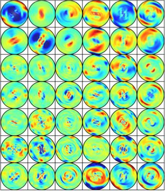
An example of this decomposition is illustrated in orthonormality of the temporal POD modes produce
Fig. 1 for a 3D plasma simulation that is dominated by
∇·χB
i = 0, ∀i. (9)
harmonics of a driving frequency. In general, examining
the structure and symmetry in the spatial and tempo- In other words, the orthonormality of the temporal
ral POD modes can inform physical understanding. For modes guarantees that the local divergence constraint
instance, in Fig. 1, the short-wavelength structures ex- is satisfied by each of the χBi by construction. In con-
hibited in the 3D spatial modes derive both from dis- trast, global energy conservation will produce strong con-
persive whistler waves via the Hall term and the small straints on the structure of the coefficients in Eq. 8.
characteristic scale associated with the driving actuator.
The steep fall-off in the singular values also indicates that
models of only the first few modes would be enough to A. Global conservation of energy
accurately forecast and control the dominant dynamics.
For an examination of the global conservation laws, we
consider isothermal Hall-MHD with the assumption that
the density is slowly-varying in time. This model reduces
to ideal MHD and incompressible resistive or Hall MHD
C. POD-Galerkin models in the appropriate limits, and produces (Galtier [39] Eq.
3.22)
Z
While we have obtained a useful modal decomposition ∂W 2 η 2 4 2 3
=− ν̃(∇×u) + (∇×B) + ν̃(∇·u) d x (10)
of the evolved fields, we have yet to derive a model for ∂t µ0 3
the subsequent temporal evolution of the modes. Now we "
I #
substitute Eq. (7) into a quadratically nonlinear MHD 1 2 4
− ρu +p u+P− ν̃(∇·u)u−ν̃u×(∇×u) ·n̂dS.
model, such as ideal MHD, incompressible Hall-MHD, or 2 3
compressible Hall-MHD with a slowly time-varying den-
sity. Utilizing the orthonormality of the χi produces: Here n̂ is a unit normal vector to the boundary, and
r r 1 ue η
P= E ×B = ·(B 2 I −BB)− 2 (∇×B)×B, (11)
X X
ȧi (t) = Ci0 + L0ij aj + Q0ijk aj ak , (8) µ0 µ0 µ0
j=1 j,k=1
Ci0 = hC+L(q̄)+Q(q̄, q̄), χi i, is the Poynting vector (E is the electric field), which is
often a known function of space and time. Omission of
L0ij = hL(χj )+Q(q̄, χj )+Q(χj , q̄), χi i, the Hall term changes ue to u. Even with a Hall-MHD
Q0ijk = hQ(χj , χk ), χi i. model that evolves the temperature, the electron diamag-
netic contribution to P does not change the energy bal-
The inner products integrate out the spatial dependence, ance if Dirichlet boundary conditions are used for ρ and
and the model is quadratic in the temporal POD modes T . To simplify, we assume that u· n̂=u× n̂=0, J · n̂=0,
ai (t). In contrast to Eq. (8), a Galerkin model based on and B · n̂=0 at the wall, consistent with the simulations
separate POD expansions for each field would involve sig- used in the accompanying work [16]. Moreover, we now
nificantly more complicated nonlinear terms from mixing assume that we have a steady-state, define a constant
and a lack of orthonormality hχu B
i , χj i 6= δij between the a0 (t)=1, and substitute Eq. (7) into Eq. (10).
Z " #
∇ρ ∇ρ
I
∂W η ν 2 η 2 4 ν
0≈ = ((∇×B)×B)· n̂dS − (∇×Bu − ×Bu ) + 2 (∇×B) + (∇·Bu − ·Bu ) d3 x, (12)
2
∂t µ20 µ0 2ρ µ0 3 µ0 2ρ
r
X r
X r
X r
X r X
X r r X
X r
=W C + WiL ai + WijQ ai aj =W C + ai (WiL + WijQ aj )=W C + WijQ ai aj = WijQ ai aj ,
i=1 i,j=1 i=1 j=1 i=1 j=0 i=0 j=0(a) Pairwise correlations of POD amplitudes (b) Spatial POD modes
4
a1 a2 a3 a4 a5 a6 a7 Bx By Bz Bxu Byu Bzu
a1 χ1
a2 χ2
100
a3 χ3
Normalized singular values
10−1
a4 χ4
10−2
10−3 a5 χ5
10−4
a6 χ6
10−5
0 10 20 30
Mode index a7 χ7
(c) Time evolutions a(t) and Fourier transforms ã(ω)
t a1 a2 a3 a4 a5 a6 a7
1
0
-1
1
1 2 3 4 5
0
ω ã1 ã2 ã3 ã4 ã5 ã6 ã7
FIG. 1: The first seven POD modes for an isothermal, compressible Hall-MHD simulation of the HIT-SI device [38]:
(a) Feature space trajectories of every mode pair and the singular values; (b) 3D spatial modes visualized in the
Z = 0 midplane and normalized to ±1; (c) Normalized temporal modes and corresponding Fourier transforms
produce harmonics of the driving frequency, labeled 1-5 in the Fourier space.
Q Q Q
where we have padded the matrix in the last step so that W0i =0, Wi0 =WiL for i∈{1,...,r}, and W00 =W C . It
Q
immediately follows from Eq. (12) that Wij is an antisymmetric matrix. Writing out the coefficients we have
Z
∇ρ ∇ρ
I
Q η η 4
(∇×B̄)×B̄ ·n̂dS− ν(∇×B̄u− ×B̄u )2+ (∇×B̄)2+ ν(∇·B̄u− ·B̄u )2 d3 x,
0=W00= (13)
µ0 2ρ µ0 3 2ρ
I
Q η h i
0=Wi0 = (∇×B̄)×χBi +(∇×χ B
i )×B̄ ·n̂dS
µ0
Z
∇ρ ∇ρ Bu η 4 ∇ρ Bu ∇ρ Bu
−2 ν(∇×B̄u− ×B̄u )·(∇×χB i
u
− ×χi )+ (∇×B̄)·(∇×χ B
i )+ ν(∇·B̄ u− ·B̄u )·(∇·χi − ·χ ) d3 x,
2ρ 2ρ µ0 3 2ρ 2ρ i
I
Q η h i
Wij = (∇×χB B
i )×χj ·n̂dS
µ0
Z
Bu ∇ρ Bu Bu ∇ρ Bu η 4 Bu ∇ρ Bu Bu ∇ρ Bu
− ν(∇×χi − ×χi )·(∇×χj − ×χj )+ (∇×χi )·(∇×χj )+ ν(∇·χi − ·χi )·(∇·χj − ·χj ) d3 x.
B B
2ρ 2ρ µ0 3 2ρ 2ρ
With some algebra, we can compute ai ȧi for i∈{1,...,r}, In index notation ai ȧi =ai Ci0 +ai L0ij aj +ai Q0ijk aj ak for
Q
r i,j,k∈{1,...,r}. First, note that Wi0 =0 produces Ci0 =0
1 ∂q 2 3
Z Z
X ∂aj ∂W
ai ȧi = ai χi χj d3 x= d x= (14)
i,j=1
∂t 2 ∂t ∂t5
for all i∈{1,...,r}. In other words, there are no constant in the energy at all, meaning
terms in the Galerkin model; data-driven methods can
implement this constraint by simply searching for models aT Q0 aa=0. (16)
that do not have constant terms. This a physical conse-
quence of our assumption that q̄ is steady-state because This is the condition for a system to have energy-
nonzero constant terms in the Galerkin model would im- preserving quadratic nonlinearities; this conclusion does
ply the possibility of unbounded growth in the energy not rely on any assumption of steady-state and energy-
norm. The anti-symmetry of WijQ for i,j ∈{1,...,r} con- preserving structure in other quadratic nonlinearities is
well-studied in fluid mechanics [20, 40].
strains the quadratic structure of aT ·a,
aT L0 a≈0. (15)
B. Global conservation of cross-helicity
This physical interpretation is also clear; if the plasma is
steady-state but has finite dissipation, the input power, An analogous derivation can be done to further con-
here manifested through a purely quadratic Poynting flux strain the model-building for systems which conserve
P ∝ηJ ×B, must be balancing these losses. Finally, be- cross-helicity, although this is not appropriate for the
cause of the boundary conditions there are no cubic terms simulation results in the accompanying work [16]. Con-
sider the local form of cross-helicity Hc =u·B. Using
Galtier [39] Eq. (3.36),
!
2
∂Hc u γp di
=−∇· + B +u×(u×B)− √ u× (∇×B)×B −ηu×(∇×B) (17)
∂t 2 (γ −1)ρ ρµ0
4 di
+ν∇· B ×(∇×u)+ (∇·u)B − √ (∇×u)· (∇×B)×B −(η+ν)(∇×B)·(∇×u).
3 ρµ0
Consider again the simplifying case J · n̂=0, B · n̂=0, and u· n̂=u× n̂=0. Then the integral form is
Z " #
∇ρ
Z
∂Hc 3 4 di
(∇×u)· (∇×B)×B −(η+ν)(∇×B)·(∇×u) d3 x. (18)
0≈ d x= ν · B×(∇×u)+ (∇·u)B − √
∂t ρ 3 ρµ0
Substituting in Eq. (7) produces terms up to cubic in the compatible with) our constraint on the energy-preserving
temporal POD modes, nonlinearities in Eq. (16). The simplest solution is
Z Z Aij Q0jkl =0 for all i,k,l, since this corresponds to standard
∂Hc 3 ∂ 1 MHD without the Hall term. Like the analysis of the lin-
d x= (ai aj ) √ χBu ·χB 3
j d x (19)
∂t ∂t ρµ0 i ear terms, this constraint indicates that if the Hall-terms
have this special energy-preserving structure, nonzero
0
∂ Aij Cj ai
Hall contributions can still conserve cross-helicity. En-
0=Aij (ai aj )= Aij L0jk ai ak forcing other invariants of Hall-MHD may require alter-
∂t A Q0 a a a
ij jkl i k l native formulations to the one presented here, since de-
rived fields like the vector potential are involved.
Note that if the system is energy-preserving, Cj0 =0 for
all j, so the first equality is already satisfied. The second
inequality gives Aij L0jk anti-symmetric under swapping i
and k, and energy-preservation gave anti-symmetry un- C. Conservation laws with velocity units
der swapping j and k (Eq. 15). The most straightforward
solution is L0jk =0 for all j,k; this solution is precisely the In closer analogy to fluid dynamics [17], we could have
ideal limit corresponding to η=ν =0. Since Aij is not alternatively used q=[u,uA ,us ],
symmetric by construction, this constraint can also ap-
ply to systems which conserve cross-helicity despite finite 4T B
u2s = , uA = √ , (20)
dissipation. mi (γ −1) µ0 ρ
Z
Lastly, Aij Q0jkl , containing only the contribution from 1 1 2
hq,qi= u +u2A +u2s d3 x. (21)
the Hall-term, exhibits the same structure as (and is 2 26
We have defined a scaled plasma sound speed, us . If rithms can directly incorporate global conservation laws
ρ is uniform ρhq,qi/2=W . The isothermal and time- during the search for low-dimensional models in plasma
independent density assumptions allow us to derive an- datasets. We use the sparse identification of nonlinear
other quadratic model in q, for which a POD-Galerkin dynamics (SINDy) algorithm [47] to identify nonlinear
model is readily available (the form is identical to Eq. 8 reduced-order models for plasmas in the accompanying
but the coefficients have changed). Once again, assume work [16].
u· n̂=u× n̂=0, and B · n̂=0 on the boundary, so that
ρ dq 2 3
Z
∂W
d x= . (22) A. The constrained SINDy method
2 dt ∂t
This is equivalent to Eq. (14) in the particular case of The goal of SINDy is to identify a low-dimensional
time-independent density. Without this R assumption, an model for a(t), the vector of POD amplitudes, as a sparse
extra term appears, proportional to u·∇(u2 +u2A )d3 x. linear combination
Although from dimensional analysis this term is poten- of elements from alibrary of candi-
date terms Θ= θ1 (a) θ2 (a) ··· θp (a) :
tially very large, this may not be the case for many lab-
oratory devices with strong anisotropy introduced by a d
large external magnetic field. For instance, steady-state a=f (a)≈Θ(a)Ξ. (23)
dt
toroidal plasmas with large closed flux surfaces would
expect u·∇u2A and u·∇u2 to be small, as the fluid ve- To address this combinatorically hard problem, it lever-
locity is primarily along field lines and gradients in both ages sparse regression techniques, optimizing for the
the magnetic and velocity fields are primarily across field sparsest set of equations that produces an accurate fit
lines. For this reason, in certain devices the use of of the data. The SINDy optimization problem is
q=[u,uA ,us ] could be a useful alternative to the formu-
lation used in the main body of this work. It is possi- minΞ ||ȧ−Θ(a)Ξ||22 +λR(Ξ), (24)
ble that, in these units, the structure of the nonlinear- subject to DΞ[:]=d,
ities in the associated POD-Galerkin model may prove
more amenable to analysis. Now that we have illustrated where R(Ξ) is some regularizer, like the L0 or L1
how global conservation laws manifest as structure in norm, which promotes sparsity in Ξ. Here a, ȧ∈
Galerkin models, we could compute these coefficients and RM ×r , Θ(a)∈RM ×N , Ξ∈RN ×r , D∈RNc ×rN , Ξ[:]∈
evolve the subsequent model. However, For an explicit RrN , d∈RNc , where N is the number of candidate
calculation of the model coefficients, the first and sec- terms,
a1 Nc is the number of constraints, and Ξ[:]=
ond order spatial derivatives for the MHD fields must be ξ1 ··· ξ1ar ··· ξN
a1 ar
··· ξN .
well-approximated in the region of experimental interest.
In some cases, high-resolution diagnostics on experimen-
tal devices can resolve these quantities in a particular
region of the plasma, but even if this data is available, B. Derivation of the SINDy constraints
computing these inner products and evaluating the non-
linear terms in the model is resource-intensive. Fortu- In Sec. III, we derived model constraints from global
nately, there are hyper-reduction techniques from fluid conservation laws; our goal here is to rewrite these con-
dynamics [41], such as the discrete empirical interpola- straints to be compatible with the notation in Eq. 24.
tion method (DEIM) [42], QDEIM [43], missing-point es- The conclusions for the global conservation of energy
timation (MPE) [44] and gappy POD [45, 46], which can were: 1) no constant terms, 2) an anti-symmetry
enable efficient computations. Instead of using hyper- constraint on the linear part of the coefficient ma-
reduction, one can use emerging and increasingly sophis- trix Ξ, and 3) a more complicated energy-preserving
ticated machine learning methods to discover Galerkin structure in the quadratic coefficients. Consider a
models from data. In the following section, we derive quadratic library in a set of r modes, ordered as Θ(a)=
constraints on machine learning methods that guarantee [a1 ,...,ar ,a1 a2 ,...,ar−1 ar ,a21 ,...,a2r ]. Note that this ar-
the model structure we derived from global conservation rangement of the polynomials in Θ differs from Loiseau
laws in Sec. III. et al. [40], so the indexing and subscripts are also dif-
ferent here. First we will consider the constraint on the
linear part of the Galerkin model in Eq. 8, or equivalently
that the quadratic term aT L0 a≈0. We can rewrite this
IV. GLOBAL CONSERVATION LAWS IN
MACHINE LEARNING MODEL DISCOVERY
in the SINDy notation as
a1
··· ξra1 a1
ξ
1. .
Increasingly, machine learning techniques are allowing . . ... .
0= a1 ··· ar .. .. . (25)
scientists to extract a system’s governing equations of
motion directly from data. Here we show how these algo- ξrar ··· ξrar ar7
a a
We conclude ξi j =−ξjai for i,j ∈{1,...,r} and identify ξi j while the third type of constraint produces
by accessing the (i−1)r+j index in Ξ[:]. Note we are
only accessing the first r2 elements of Ξ[:]. For mod- ξ˜ijk +ξ˜jik +ξ˜kij =0. (31)
els limited to linear and quadratic polynomials, N =
(r2 +3r)/2 and the number of constraints from anti- This relation is equivalent to the energy-preserving con-
symmetry of the linear coefficients is NL =(r2 +r)/2. ditions in Schlegel et al. [20], but the indexing is not
Thus there are now only rN −NL =r(r2 +2r−1)/2 free straightforward, even after fully expanding Eq. 28. This
parameters. Since the constrained SINDy algorithm equation is an arbitrary r generalization to the r=3 con-
solves linear equality constraints of the form DΞ[:]=d, straint used in Loiseau et al. [40]. For the specific case
we can write this out explicitly for r=3, where the plasma system is Hamiltonian (for instance
in ideal [48], Hall [49], and extended [50] MHD without
dissipation) and the measurements are assumed to be
1 0 0 0 0 0 0 0 0 0 ··· ξ1a1 0
0 0 0 0 1 0 0 0 0 0 ··· a2 0 sufficient to represent the Hamiltonian, one could alter-
ξ1 natively use formulations of SINDy to directly discover
0 0 0 0 0 0 0 0 1 0 ··· ξ a3 0
1 = . (26) the Hamiltonian [51] and subsequently derive the equa-
0 1 0 1 0 0 0 0 0 0 ··· ξ2a1
0
tions of motion. Lastly, cross-helicity constraints can
0 0 1 0 0 0 1 0 0 0 ··· . 0
.. be straightforwardly implemented from these results. If
0 0 0 0 0 1 0 1 0 0 ··· 0
the constraint on the quadratic terms in Ξ is written
The boundary conditions u·n̂=0, J ·n̂=0, B·n̂=0 guar- Djk Ξk =0, then the quadratic cross-helicity constraint
anteed that the quadratic nonlinearities were energy- can be written Djk Akl Ξl =0.
preserving, and thus that cubic terms in Eq. 10 vanish.
In this case, regardless of the steady-state assumption,
V. CONCLUSION
we have that
r
X A hierarchy of models with varying fidelity is essen-
Q0ijk ai aj ak ≈0. (27) tial for understanding and controlling plasmas. The
i,j,k=0
present work, along with the accompanying work [16],
This constraint is significantly more involved to reformat. provides a principled lower level on this hierarchy − low-
Written in SINDy notation, this is equivalent to dimensional and interpretable plasma models which can
be used for physical discovery, forecasting, stability anal-
ysis, and real-time control. We have illustrated how
a1 a2
a1 .. Galerkin plasma models retain the global conservation
a1 a1
ξr+1 ξr+2 ··· ξN . laws of MHD, and how machine learning methods like
.
0= a1 ··· ar .. .. .. .. ar−1 ar
SINDy can use these constraints directly in an optimiza-
. . . a21 . (28)
ar ar ar tion procedure for discovering such models from data.
ξr+1 ξr+2 ··· ξN .
.. This principled enforcement of global conservation laws
is critical for the success of future low-dimensional plasma
a2r
models.
Expand this all out and group the like terms, i.e. terms
which look like a3i , ai a2j or ai aj ak , i,j,k∈{1,...,r}, i6=
VI. ACKNOWLEDGEMENTS
j 6= k. All of the like terms can be straightforwardly
shown to be linearly independent, so we can consider
three constraints separately for the three types of terms. The authors would like to extend their gratitude to
The number of each of these respective terms is 1r =r, Dr. Uri Shumlak for his input on this work. This work
2 2r =r(r−1), and 3r =r(r−1)(r−2)/6, for a total of and the companion work were supported by the Army
r(r+1)(r+2)/6=NQ constraints. With both constraints, Research Office (ARO W911NF-19-1-0045) and the Air
we have rN −NL −NQ =r(r−1)(2r+5)/6 free parameters, Force Office of Scientific Research (AFOSR FA9550-18-
and Nc =NL +NQ constraints. Further considering the 1-0200). Simulations were supported by the U.S. Depart-
quadratic case, we find that coefficients which adorn a3i ment of Energy under award numbers DE-SC0016256
must vanish, ξNai and DE-AR0001098 and used resources of the National
−r+i =0. Now define
Energy Research Scientific Computing Center, supported
by the Office of Science of the U.S. Department of Energy
ξ˜ijk =ξr+
ai
j . (29)
(2r−j−3)+k−1
2 under Contract No. DE-AC02–05CH11231.
The second type of constraint, with i6= j, produces
(
ai ξ˜jij ij,8
[1] J. Candy and R. E. Waltz, Anomalous transport scal- projection, Physica D: Nonlinear Phenomena 189, 115
ing in the DIII-D tokamak matched by supercomputer (2004).
simulation, Phys. Rev. Lett. 91, 045001 (2003). [18] B. R. Noack, M. Schlegel, M. Morzynski, and G. Tad-
[2] O. Ohia, J. Egedal, V. S. Lukin, W. Daughton, and A. Le, mor, Galerkin method for nonlinear dynamics (Springer,
Demonstration of anisotropic fluid closure capturing the 2011).
kinetic structure of magnetic reconnection, Phys. Rev. [19] M. J. Balajewicz, E. H. Dowell, and B. R. Noack, Low-
Lett. 109, 115004 (2012). dimensional modelling of high-Reynolds-number shear
[3] D. Grošelj, A. Mallet, N. F. Loureiro, and F. Jenko, Fully flows incorporating constraints from the Navier–Stokes
kinetic simulation of 3D kinetic Alfvén turbulence, Phys. equation, Journal of Fluid Mechanics 729, 285 (2013).
Rev. Lett. 120, 105101 (2018). [20] M. Schlegel and B. R. Noack, On long-term boundedness
[4] K. Taira, S. L. Brunton, S. Dawson, C. W. Rowley, of Galerkin models, Journal of Fluid Mechanics 765, 325
T. Colonius, B. J. McKeon, O. T. Schmidt, S. Gordeyev, (2015).
V. Theofilis, and L. S. Ukeiley, Modal analysis of fluid [21] K. Carlberg, M. Barone, and H. Antil, Galerkin v. least-
flows: An overview, AIAA Journal 55, 4013 (2017). squares Petrov–Galerkin projection in nonlinear model
[5] I. Furno, Fast transient transport phenomena measured reduction, Journal of Computational Physics 330, 693
by soft x-ray emission in TCV tokamak plasmas, Tech. (2017).
Rep. (2001). [22] T. Dudok de Wit, A.-L. Pecquet, J.-C. Vallet, and
[6] R. Jiménez-Gómez, E. Ascası́bar, T. Estrada, I. Garcı́a- R. Lima, The biorthogonal decomposition as a tool for
Cortés, B. Van Milligen, A. López-Fraguas, I. Pastor, investigating fluctuations in plasmas, Physics of Plasmas
and D. López-Bruna, Analysis of magnetohydrodynamic 1, 3288 (1994).
instabilities in TJ-II plasmas, Fusion science and tech- [23] J. Levesque, N. Rath, D. Shiraki, S. Angelini, J. Bialek,
nology 51, 20 (2007). P. Byrne, B. DeBono, P. Hughes, M. Mauel, G. Navratil,
[7] B. P. van Milligen, E. Sánchez, A. Alonso, M. A. Pe- et al., Multimode observations and 3D magnetic control
drosa, C. Hidalgo, A. M. de Aguilera, and A. L. Fraguas, of the boundary of a tokamak plasma, Nuclear Fusion
The use of the biorthogonal decomposition for the iden- 53, 073037 (2013).
tification of zonal flows at TJ-II, Plasma Physics and [24] C. Galperti, C. Marchetto, E. Alessi, D. Minelli,
Controlled Fusion 57, 025005 (2014). M. Mosconi, F. Belli, L. Boncagni, A. Botrugno, P. Bu-
[8] M. Pandya, Low edge safety factor disruptions in the ratti, B. Esposito, et al., Development of real-time MHD
Compact Toroidal Hybrid: Operation in the low-q regime, markers based on biorthogonal decomposition of signals
passive disruption avoidance and the nature of MHD pre- from Mirnov coils, Plasma Physics and Controlled Fusion
cursors, Ph.D. thesis, Auburn University (2016). 56, 114012 (2014).
[9] B. Victor, C. Akcay, C. Hansen, T. Jarboe, B. Nelson, [25] B. P. Van Milligen, E. Sánchez, A. Alonso, M. Pedrosa,
and K. Morgan, Development of validation metrics using C. Hidalgo, A. M. De Aguilera, and A. L. Fraguas, The
biorthogonal decomposition for the comparison of mag- use of the biorthogonal decomposition for the identifica-
netic field measurements, Plasma Physics and Controlled tion of zonal flows at TJ-II, Plasma Physics and Con-
Fusion 57, 045010 (2015). trolled Fusion 57, 025005 (2014).
[10] E. Strait, J. King, J. Hanson, and N. Logan, Spatial and [26] C. Hansen, B. Victor, K. Morgan, T. Jarboe, A. Hos-
temporal analysis of DIII-D 3D magnetic diagnostic data, sack, G. Marklin, B. Nelson, and D. Sutherland, Nu-
Review of Scientific Instruments 87, 11D423 (2016). merical studies and metric development for validation
[11] P. J. Byrne, Study of External Kink Modes in Shaped of magnetohydrodynamic models on the HIT-SI exper-
HBT-EP Plasmas, Ph.D. thesis, Columbia University iment, Physics of Plasmas 22, 056105 (2015).
(2017). [27] D. D. Schnack, D. C. Barnes, D. P. Brennan, C. C.
[12] S. Gu, B. Wan, Y. Sun, N. Chu, Y. Liu, T. Shi, H. Wang, Hegna, E. Held, C. C. Kim, S. E. Kruger, A. Y. Pankin,
M. Jia, and K. He, A new criterion for controlling edge and C. R. Sovinec, Computational modeling of fully ion-
localized modes based on a multi-mode plasma response, ized magnetized plasmas using the fluid approximation,
Nuclear Fusion 59, 126042 (2019). Physics of Plasmas 13, 058103 (2006).
[13] A. A. Kaptanoglu, K. D. Morgan, C. J. Hansen, and [28] Z. W. Ma and A. Bhattacharjee, Hall magnetohydrody-
S. L. Brunton, Characterizing magnetized plasmas with namic reconnection: The geospace environment model-
dynamic mode decomposition, Physics of Plasmas 27, ing challenge, Journal of Geophysical Research: Space
032108 (2020). Physics 106, 3773.
[14] P. Benner, V. Mehrmann, and D. C. Sorensen, Dimension [29] V. Krishan and S. M. Mahajan, Magnetic fluctuations
reduction of large-scale systems, Vol. 45 (Springer, 2005). and Hall magnetohydrodynamic turbulence in the solar
[15] P. Benner, M. Ohlberger, A. Cohen, and K. Willcox, wind, Journal of Geophysical Research: Space Physics
Model reduction and approximation: theory and algo- 109.
rithms (SIAM, 2017). [30] F. Ebrahimi, B. Lefebvre, C. B. Forest, and A. Bhat-
[16] A. A. Kaptanoglu, K. D. Morgan, C. J. Hansen, and S. L. tacharjee, Global Hall-MHD simulations of magnetoro-
Brunton, Physics-constrained, low-dimensional models tational instability in a plasma Couette flow experiment,
for mhd: First-principles and data-driven approaches, Physics of Plasmas 18, 062904 (2011).
arXiv preprint arXiv:2004.10389 (2020). [31] N. M. Ferraro, Calculations of two-fluid linear response to
[17] C. W. Rowley, T. Colonius, and R. M. Murray, Model non-axisymmetric fields in tokamaks, Physics of Plasmas
reduction for compressible flows using POD and Galerkin 19, 056105 (2012).9
[32] A. A. Kaptanoglu, T. E. Benedett, K. D. Morgan, C. J. Conference (IEEE, 2009) pp. 4316–4321.
Hansen, and T. R. Jarboe, Two-temperature effects in [43] Z. Drmac and S. Gugercin, A new selection operator for
Hall-MHD simulations of the HIT-SI experiment, Physics the discrete empirical interpolation method—improved
of Plasmas 27, 072505 (2020). a priori error bound and extensions, SIAM Journal on
[33] S. L. Brunton and J. N. Kutz, Data-driven science and Scientific Computing 38, A631 (2016).
engineering: Machine learning, dynamical systems, and [44] P. Astrid, S. Weiland, K. Willcox, and T. Backx, Missing
control (Cambridge University Press, 2019). point estimation in models described by proper orthog-
[34] G. H. Golub et al., Matrix computations, The Johns Hop- onal decomposition, IEEE Transactions on Automatic
kins (1996). Control 53, 2237 (2008).
[35] A. Frieze, R. Kannan, and S. Vempala, Fast Monte-Carlo [45] K. Willcox, Unsteady flow sensing and estimation via the
algorithms for finding low-rank approximations, Journal gappy proper orthogonal decomposition, Computers &
of the ACM (JACM) 51, 1025 (2004). Fluids 35, 208 (2006).
[36] E. Liberty, F. Woolfe, P.-G. Martinsson, V. Rokhlin, [46] K. Carlberg, C. Farhat, J. Cortial, and D. Amsallem, The
and M. Tygert, Randomized algorithms for the low-rank GNAT method for nonlinear model reduction: effective
approximation of matrices, Proceedings of the National implementation and application to computational fluid
Academy of Sciences 104, 20167 (2007). dynamics and turbulent flows, Journal of Computational
[37] F. Woolfe, E. Liberty, V. Rokhlin, and M. Tygert, A fast Physics 242, 623 (2013).
randomized algorithm for the approximation of matrices, [47] S. L. Brunton, J. L. Proctor, and J. N. Kutz, Discover-
Applied and Computational Harmonic Analysis 25, 335 ing governing equations from data by sparse identifica-
(2008). tion of nonlinear dynamical systems, Proceedings of the
[38] T. Jarboe, W. Hamp, G. Marklin, B. Nelson, R. O’Neill, National Academy of Sciences 113, 3932 (2016).
A. Redd, P. Sieck, R. Smith, and J. Wrobel, Spheromak [48] P. J. Morrison and J. M. Greene, Noncanonical hamil-
formation by steady inductive helicity injection, Physical tonian density formulation of hydrodynamics and ideal
review letters 97, 115003 (2006). magnetohydrodynamics, Physical Review Letters 45, 790
[39] S. Galtier, Introduction to modern magnetohydrodynam- (1980).
ics (Cambridge University Press, 2016). [49] Z. Yoshida and E. Hameiri, Canonical hamiltonian me-
[40] J.-C. Loiseau, B. R. Noack, and S. L. Brunton, Sparse chanics of hall magnetohydrodynamics and its limit
reduced-order modeling: sensor-based dynamics to full- to ideal magnetohydrodynamics, Journal of Physics A:
state estimation, Journal of Fluid Mechanics 844, 459 Mathematical and Theoretical 46, 335502 (2013).
(2018). [50] H. M. Abdelhamid, Y. Kawazura, and Z. Yoshida, Hamil-
[41] P. Benner, S. Gugercin, and K. Willcox, A survey of tonian formalism of extended magnetohydrodynamics,
projection-based model reduction methods for paramet- Journal of Physics A: Mathematical and Theoretical 48,
ric dynamical systems, SIAM review 57, 483 (2015). 235502 (2015).
[42] S. Chaturantabut and D. C. Sorensen, Discrete empirical [51] H. K. Chu and M. Hayashibe, Discovering interpretable
interpolation for nonlinear model reduction, in Proceed- dynamics by sparsity promotion on energy and the la-
ings of the 48th IEEE Conference on Decision and Con- grangian, IEEE Robotics and Automation Letters 5,
trol (CDC) held jointly with 2009 28th Chinese Control 2154 (2020).You can also read