Learning Multimodal Rewards from Rankings - arXiv
←
→
Page content transcription
If your browser does not render page correctly, please read the page content below
Learning Multimodal Rewards from Rankings
                                                    Vivek Myers †     Erdem Bıyık ‡       Nima Anari †       Dorsa Sadigh †,‡
                                                             †
                                                               Department of Computer Science, Stanford University
                                                           ‡
                                                             Department of Electrical Engineering, Stanford University
                                                    {vmyers,ebiyik}@stanford.edu, {anari,dorsa}@cs.stanford.edu

                                                  Abstract: Learning from human feedback has shown to be a useful approach in
                                                  acquiring robot reward functions. However, expert feedback is often assumed to
                                                  be drawn from an underlying unimodal reward function. This assumption does
arXiv:2109.12750v1 [cs.LG] 27 Sep 2021

                                                  not always hold including in settings where multiple experts provide data or when
                                                  a single expert provides data for different tasks—we thus go beyond learning a
                                                  unimodal reward and focus on learning a multimodal reward function. We formu-
                                                  late the multimodal reward learning as a mixture learning problem and develop
                                                  a novel ranking-based learning approach, where the experts are only required to
                                                  rank a given set of trajectories. Furthermore, as access to interaction data is often
                                                  expensive in robotics, we develop an active querying approach to accelerate the
                                                  learning process. We conduct experiments and user studies using a multi-task vari-
                                                  ant of OpenAI’s LunarLander and a real Fetch robot, where we collect data from
                                                  multiple users with different preferences. The results suggest that our approach
                                                  can efficiently learn multimodal reward functions, and improve data-efficiency
                                                  over benchmark methods that we adapt to our learning problem.

                                                  Keywords: HRI, reward learning, multi-modality, rankings, active learning

                                         1   Introduction
                                         Learning a reward function from different sources of human
                                         data is a fundamental problem in robot learning. In recent
                                         years, there has been a large body of work that learns reward
                                         functions using various forms of human input, such as expert
                                         demonstrations [1], suboptimal demonstrations [2, 3, 4], pair-
                                         wise comparisons [5, 6], physical corrections [7, 8], rankings
                                         [9], and trajectory assessments [10]. These works focus on
                                         learning a unimodal reward function that models human pref-
                                         erences on a target task. However, this unimodality assump-
                                         tion does not always hold: human preferences are usually more
                                         complex and need to be captured via a multimodal representa-
                                         tion. Further, even if the preferences of a human are truly uni-
                                         modal, we often use a mixture of data from multiple humans,
                                         which can be difficult to disentangle, leading to multimodality.
                                                                                                              Figure 1: Fetch robot putting a banana
                                         As an example, consider a robot placing a banana on one of on one of the three shelves. The two
                                         the three shelves (see Fig. 1). The middle shelf is often used users have different preferences, and
                                         for fruits, but it has no room left and if the robot tries to put the so they provide different rankings to
                                         banana there, it may cause other fruits to fall. The top shelf has the robot. The robot needs to be able
                                                                                                               to model multimodal reward functions
                                         some space but it has been used for cooked meals. The bottom for successfully achieving the task.
                                         shelf has a lot of free space, but is usually used only for toys.
                                         In such a scenario, people may have very different preferences about what the robot should do. If
                                         we try to learn a unimodal reward using data collected from multiple people, the robot is likely to
                                         fail in the task, because the data will include inconsistent preferences.
                                         One solution is of course to label the different modes in the data. For example, one could separate the
                                         data based on the preferred shelf, and learn different reward functions for each shelf. However, this
                                         separation is not always straightforward. For example in a driving dataset, it is unclear what should
                                         be labeled as aggressive or timid driving. Clustering the data based on the human who provided

                                         5th Conference on Robot Learning (CoRL 2021), London, UK.
the data is also not viable as it will introduce data-inefficiency issues, and perhaps more importantly,
humans are not always unimodal: a usually timid driver can drive more aggressively when in a hurry.
These examples motivate us to develop methods that can learn multimodal reward functions us-
ing datasets that are not specifically labeled with the modes. To this end, previous work proposed
learning from demonstrations to learn multimodal policies [11, 12] or reward functions with multi-
ple possible intentions [13, 14]. However, learning from expert demonstrations is often extremely
challenging in robotics as providing demonstrations on a robot with high degrees of freedom is non-
trivial [5, 15], and humans have difficulty giving demonstrations that align with their preferences
due to their cognitive biases [16, 17]. Thus, it is desirable to have methods that learn from other
more reliable sources of data. For instance, humans can reliably compare two different trajectories,
enabling a robot to learn from pairwise comparisons [5, 9, 18].
While learning from pairwise comparisons provides a rich source of data for learning reward func-
tions, the theoretical results by Zhao et al. [19] imply that extending the existing comparison-based
reward learning techniques to multimodal reward functions is not possible, i.e. failure cases can be
constructed, where pairwise comparisons are not sufficient for identifying different modes of a mul-
timodal function. Our insight is that it is possible to learn a multimodal reward function by going
beyond pairwise comparisons and instead using rankings.
To achieve this, we formulate multimodal reward learning as a mixture learning problem. As data
is a very expensive resource in robotics, we further develop an active querying method that aims to
ask the human users the most informative queries. Our contributions are three-fold:
    • We develop a method that uses rankings from humans to learn multimodal reward functions.
    • We develop an active querying method to improve data-efficiency by asking the most informative
      ranking queries.
    • We conduct extensive experiments and user studies with OpenAI’s LunarLander and a real Fetch
      robot to test our learning and querying methods in comparison to baselines.
2     Related Work
Reward Learning in Robotics. Learning reward functions from human feedback is a fundamental
problem in robot learning. Ng and Russell [20] and Abbeel and Ng [21] introduce the problem
of learning from demonstrations in the space of robotics. Later works focus on improving inverse
reinforcement learning algorithms by reducing the ambiguity in learned rewards [1, 22].
Due to the difficulty in providing expert demonstrations in robotics, recent works attempt to learn
reward functions using other forms of human feedback, such as physical corrections [7, 8] and pair-
wise comparisons where a human user compares the quality of two robot trajectories [23, 24, 25, 26].
Later works extend these algorithms for better time and data-efficiency [27, 28, 29]. Though there
have been works to extend this framework to reward functions modeled with Gaussian processes to
capture nonlinearities [6, 30, 31], the underlying reward function has always been unimodal.
Preference-based Learning. Outside of robotics, preference-based learning, where data are in the
form of comparisons, selections out of a set, or rankings, has attracted attention due to the ease of
collecting data and its reliability. Prior works have studied this in the classification [32], bandits
[33], and reinforcement learning settings [34].
In our problem, we have a continuous hypothesis space of reward functions. In such cases, it is
common to model human comparisons or rankings with a computational model. Bradley-Terry is
one such model for pairwise comparisons [35], which is easily extended to the queries where the
human chooses the best of multiple items. Known as multinomial logits (MNL) [36], this model has
been widely used for human preferences in many fields [37, 38, 39] including robotics [25, 27, 18].
To extend these models to rankings, Plackett-Luce [40, 41] and Mallows models [42, 43, 44, 45] are
commonly employed. In this paper, we use the Plackett-Luce model as it is a natural extension of
MNL, which is widely used in robotics with great success. We formalize this model in Section 3.
Even though there has been much research in this domain, all works we mentioned here focus on
the unimodal case, and do not work with the multimodal preferences.
Learning Mixture Models from Rankings. One way to model multimodal reward functions is
through mixture models, where the data is assumed to come from different individual models with
some unknown probabilities. To this end, previous works consider mixtures of MNLs [46, 47],

                                                   2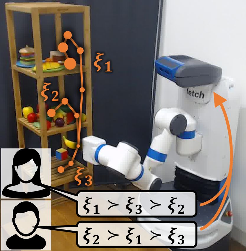
Plackett-Luce models [19], and Mallows models [48]. Other works adopt different methods to
model multimodality, such as by assuming latent state dynamics that transition between different
modes [49, 50] or by learning the different modes from labeled datasets [51, 52]. To avoid these
modeling assumptions, we focus on directly learning the mixture model.
While Zhao et al. [19] have theoretically studied the mixture of Plackett-Luce choice models, which
also informs our algorithm in terms of the query sizes, they only focus on learning the rewards of
a discrete set of items. To the best of our knowledge, our paper is the first work that deals with a
continuous hypothesis space under a mixture of Plackett-Luce models. Furthermore, we propose
an active querying strategy for this mixture model to improve data-efficiency for human-in-the-loop
learning, which is crucial in data-hungry applications such as robotics.
3    Problem Formulation
Setup. We consider a fully-observable deterministic dynamical system. A trajectory ξ in this system
is a series of states and actions, i.e., ξ = (s0 , a0 , . . . , sT , aT ). The set of feasible trajectories is Ξ.
We assume there is a set of M individual reward functions that are possibly different, each of which
encodes some preference between the trajectories in Ξ. For the rest of the formalism, we refer to
each individual reward function as an expert for the clarity of the presentation.
Following the common linearity assumption in reward learning [1, 5, 28], we assume each preference
can be modeled as a linear reward function over a known fixed feature space Φ, so the reward
                                                                            ⊤
associated with a trajectory ξ with respect to the mth expert is Rm (ξ) = ωm  Φ(ξ), where ωm is the
unknown vector of weights. Across the expert population, there exists some unknown distribution
over the reward parameters, corresponding to the ratio of the data provided by the experts. We
                                                                  ∑︁M
represent this distribution with mixing coefficients αm such that m=1 αm = 1. We will then learn
both the unknown reward functions {ωm }M                                        M
                                           m=1 and the mixing coefficients {αm }m=1 , using ranking
queries made to the M experts. This setup generalizes [5], which studied unimodal rewards.
Ranking Model. We define a ranking query to be a set of the form Q = {ξ1 , . . . , ξK } for a fixed
query size K. The response to a ranking query is a ranking over the items contained therein, of the
form x = (ξa1 , . . . , ξaK ), where a1 is the index of the expert’s top choice, a2 is the second top choice,
and so on. While it is not known which expert provided the response to the query, we know the prior
that a response comes from expert m with some unknown probability αm , i.e., Pr(R = Rm ) = αm .
Going back to our banana placing example, a ranking query of K robot trajectories is generated by
the algorithm, and a user—whose identity is unknown to the algorithm—responds to this query.
We then capture how human experts respond to these ranking queries by modeling a ranking dis-
tribution through an iterative process using Luce’s choice axiom [53]. In this process, the experts
repeatedly select their top choice am with a probability distribution generated with the softmax rule
to generate a ranking from the order items were selected:
                                                                eRm (ξa1 )
                            Pr (x1 = ξa1 | R = Rm ) = ∑︁K R (ξ ) .
                                                                      m aj
                                                               j=1 e
In the following iterations, the experts select their top choice among the remaining trajectories:
                                                                       eRm (ξai )
                     Pr (xi = ξai | x1 , . . . , xi−1 , R = Rm ) = ∑︁K R (ξ ) .                    (1)
                                                                             m aj
                                                                      j=i e
This is known as the Plackett-Luce ranking model [40, 41]. Together with the prior over experts αm ,
the resulting distribution over rankings x ∼ X is a mixture of Plackett-Luce models with mixing
coefficients αm and weights proportional to eRm (ξ) .
Hence, the ranking distribution first selects the reward function Rm with probability αm , and then
selects trajectories from Q sequentially with probability proportional to the exponent of their reward,
i.e., eRm , among the remaining trajectories until none is left, generating a ranking of the trajectories.
So given knowledge of the true reward function weights ωm and mixing coefficients αm , we have
the following joint mass over observations x from a query Q:
                                          M       K        ⊤
                                         ∑︂      ∏︂      eωm Φ(ξai )
                           Pr(x | Q) =        αm     ∑︁K ωm   ⊤ Φ(ξ       .                (2)
                                                                     aj )
                                         m=1     i=1    j=i e

                                                       3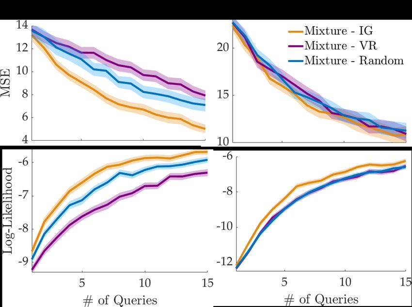
Objective. Our goal is to design a series of adaptive queries Q(t) to optimally learn the reward
weights ωm and corresponding mixing coefficients αm upon observing the query responses x(t) .
We constrain all queries to consist of a fixed number of elements K.
4     Active Learning of Multimodal Rewards from Rankings
In this section, we first start with presenting our learning framework. We then discuss how we can
improve data-efficiency, and propose an active querying approach.
4.1   Learning from Rankings
To learn the reward weights ωm and mixing coefficients αm , we adopt a Bayesian learning approach.
For this, we maintain a posterior over the parameters ωm and αm . Denoting the distribution over the
parameters αi and ωi as Θ, this posterior can be written(︂       as                )︂
  Pr(Θ | Q , x , Q , x , . . . ) ∝ Pr(Θ) Pr Q , x(1) , Q(2) , x(2) , · · · | Θ
             (1)  (1)    (2)   (2)                           (1)

          ∏︂ (︂                                                     )︂       ∏︂ (︂              )︂
= Pr(Θ)       Pr x(t) , Q(t) | Θ, Q(1) , x(1) , ..., Q(t−1) , x(t−1) ∝ Pr(Θ)   Pr x(t) | Θ, Q(t) , (3)
          t                                                              t
where we use the conditional independence of ranking queries x(t) given Θ and the conditional
independence of the Q(t) on Θ given Q(1) , x(1) , . . . , Q(t−1) , x(t−1) in the last equation. To be
able to compute this posterior, we assume some prior distribution over the reward weights and the
mixing coefficients, which is system-dependent and may come from domain knowledge, and use
Eq. (2) to calculate the likelihood terms. For example, in our simulations and user studies, we
adopted a Gaussian prior ωi ∼ N (0, I) and a uniform prior α ∼ Unif(∆M −1 ) where ∆M −1 is the
unit M − 1 simplex. Learning this posterior distribution in Eq. (3), one can compute a maximum
likelihood estimate (MLE) or expectation as the predicted reward weights and mixing coefficients.
Equation (3) implies the queries made to the experts, Q(t) ’s, affect how well the posterior will
be learned. Assuming a limited budget of queries, which is often the case in many real-world
applications, including robotics, one would ideally find an optimal adaptive sequence of queries such
that the responses would give the highest amount of information about the reward weights and the
mixing coefficients. However, this is NP-hard, even in the unimodal case with pairwise comparisons
[54]. We therefore resort to greedy optimization techniques to develop our active learning approach.
4.2   Active Querying via Information Gain
A query Q is desirable if observing its value x yields high information about the underlying model
parameters, αm and ωm . Therefore, we propose using an information gain objective to adaptively
select the most informative query at each querying step, generalizing the approach of [5].
                                                                                    {︁ ′     ′ }︁t−1
Assume at a fixed timestep t we have made past query observations D = Q(t ) , x(t ) t′ =1 .
The desired query is then Q∗ = arg maxQ I(Q; Θ | D) where I(·; ·) denotes mutual informa-
tion. Equivalently, denoting conditional entropy with H[· | ·] and the joint distribution over x and
                M
θ = {αm , ωm }m=1 conditioned on Q and D as P (X, Θ | Q, D), we see
                                                     Eθ′ ∼Θ|D Pr [X = x | Q, θ′ ]
                     Q∗ = arg min         E      log                              .                (4)
                               Q     P (X,Θ|Q,D)          Pr[X = x | Q, θ]
The details of this derivation are presented in Appendix A.
4.3   Overall Algorithm
To efficiently solve the optimization in Eq. (4), we first note that we should use a Monte Carlo
approximation since the expectations are taken over a continuous variable Θ and a discrete variable
X over an intractably large set of K! alternatives. To perform this Monte Carlo integration, we
require samples from the posterior Pr(X, Θ | Q, D).
Our key insight is that we can obtain joint
                                       (︁ samples from)︁ both posteriors by first sampling from Θ̄ ∼
Pr(Θ | D) and then sampling(︁x ∼ Pr X | Q,)︁ Θ = Θ̄ since Θ ⊥ Q | D and X ⊥ D | Q, Θ. We
perform the sampling x ∼ Pr X | Q, Θ = Θ̄ efficiently using Eq. (2). In general, exact sampling
from the posterior Pr(Θ | D) is intractable. However, we note Eq. (3) can be directly evaluated
(using Eq. (2)) and gives Pr(Θ | D) up to a proportionality constant factor.
With this unnormalized posterior of Eq. (3), we use the Metropolis-Hastings algorithm as described
in Appendix B to generate samples from the posterior Pr(Θ | D).

                                                  4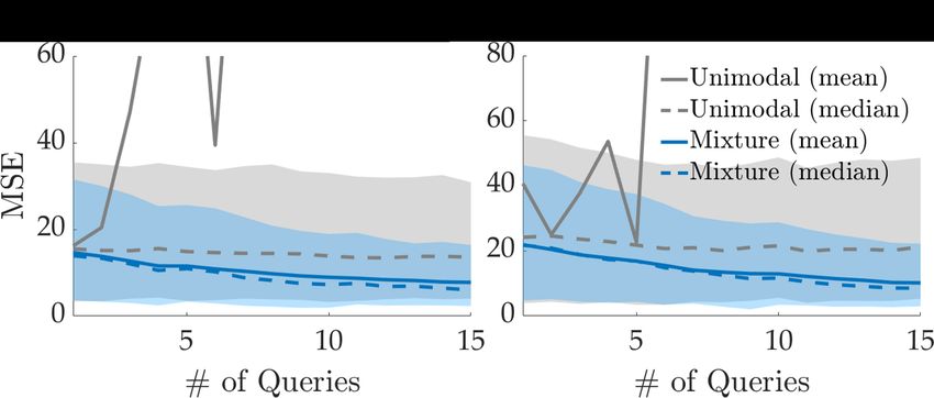
We see our optimization problem   (︁ simplifies)︁ to finding, for N fixed samples θ̄i ∼ Pr(Θ | D) and
corresponding samples: xi ∼ Pr X | Q, θ̄i
                N [︃       N
                        (︂∑︂                                         ]︃
               ∑︂                          ]︁)︂
                             Pr xi | Q, θ̄j −log Pr xi | Q, θ̄i , Q∗ = arg min L(Q; x, θ̄) . (5)
                               [︁                        [︁        ]︁
 L(Q; x, θ̄) =      log
               i=1       j=1                                                     Q

We solve this optimization using Algorithm 1 Active Querying via Information Gain
simulated annealing [55] (see Ap-
pendix C). Algorithm 1 goes over Require:               Observations D
the pseudocode of our approach, and 1: θ̄i N ∼ Pr(Θ | D) w/ Eq. (3) via Metropolis-Hastings
                                                 {︁ }︁
                                                       i=1
we discuss the hyperparameters in 2: procedure E VAL            (︁ Q UERY(Q))︁
our experiments in Appendix D.            3:        ∀i, xi ∼ Pr xi | Q, θ̄i
4.4 Analysis                              4:        return L(Q; x, θ̄)                          ▷ Eq. (5)
                                          5: end procedure
We start the analysis by stating the 6: Q ← M INIMIZE(E VAL Q UERY) ▷ Simulated annealing
bounds on the required number of 7: select query Q
trajectories in each ranking query to
achieve generic identifiability. A Plackett-Luce model over Ξ is generically identifiable if for any
sets of parameters Θ1 and Θ2 inducing the same distribution over the responses to all queries of
size K on Ξ, the mixing coefficients of Θ1 and Θ2 are the same and the induced rewards Rm (ξ) are
identical across Ξ up to a constant additive scaling factor.
Theorem 1 (Zhao et al. [19]). A mixture    ⌋︁of M Plackett-Luce models with query size K and |Ξ| = K
is generically identifiable if M ≤ K−2
                                    ⌊︁
                                       2      !.
This statement follows directly from [19], which proves the above bound assuming that each query
to the Plackett-Luce mixture is a full ranking over the set of items (i.e. |Ξ| = K). However, the
assumption |Ξ| = K is untenable in the active learning context, as it prevents any active query
selection. To apply this result for our active learning algorithms, we relax the condition to |Ξ| ≥ K.
Corollary⌊︁ 1.1.⌋︁ A mixture of M Plackett-Luce models with query size K is generically identifiable
if M ≤ K−2  2     !.
We prove Corollary 1.1 in Appendix E.1. In our context, generic identifiability implies if the human
response is modelled by a Plackett-Luce mixture, our Algorithm 1 will be able to recover its true
parameters (up to a constant additive factor for the rewards) in the limit of infinite queries.
Remark 1. Greedy selection of queries maximizing information gain in Eq. (4) is not necessarily
within a constant factor of optimality.
Appendix E.2 justifies Remark 1. In fact, greedy optimization of information gain for adaptive active
learning can be significantly worse than a constant factor of optimality in pathological settings [56].
Despite its lack of theoretical guarantees, information gain is a commonly used effective approach
in adaptive active learning [29, 57, 58]. Although other approaches like volume removal satisfy
adaptive submodularity [25], they fail in settings with noisy observations by selecting high-noise
low-information queries, and in practice achieve far worse performance than information gain.
5   Experiments
Having presented our learning and active
querying algorithms, we now evaluate their per-
formance in comparison with other alternatives.
We start with describing the two tasks we ex-
perimented with:
LunarLander. We used 1000 trajectories in
OpenAI Gym’s LunarLander environment [59] Figure 2: The LunarLander environment is visualized
                                                 with the two tasks. Sample trajectories associated with
shown in Fig. 2 (see Appendix G.1 for details these tasks are shown.
on how they were generated).
Fetch Robot. We generated 351 distinct trajectories of the Fetch robot [60] putting the banana on
the shelves as shown in Fig. 1 (see Appendix G.2 for details).
5.1 Methods
We compare our active querying via information gain (IG) discussed in Algorithm 1 with two base-
lines: A simple benchmark for active learning is random query selection without replacement. We
also benchmark against volume removal (VR), a common objective for active learning of robot re-
ward functions [25]. See Appendix F for the details of these two baselines.

                                                   5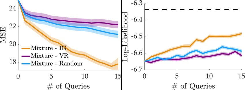
5.2       Metrics
We want to evaluate both the active querying and the learning performance.
                                                                       {︁        The}︁ former requires
metrics that assess the quality of the algorithm’s selected queries D = (Q(t) , x(t) ) t in terms of the
information they provide on the model parameters Θ. We use two such metrics: mean squared error
(MSE) and log-likelihood. Since both active and non-active methods are expected to reach the same
performance with a large number of queries, we look at the area under the curve (AUC) of these two
metrics over number of queries. To evaluate the learning performance, we quantify the success of a
robot, which learned a multimodal reward, via the learned policy rewards on the actual task.
MSE. Suppose we know the human is truly modeled by Θ∗ adhering to the assumed model class
of Section 3. Given a set of observations D, we can compute an MLE estimate Θ     ˆ︁ of the model
                                                                            ∗
parameters using Eq. (2). The MSE is then the squared error between Θ
                                                                    ˆ︁ and Θ (see Appendix H.1).
While this metric cannot be evaluated with real humans, we can use this metric with synthetic human
models (model with known parameters Θ∗ ) in simulation. A lower MSE score means the selected
queries D allow us to better learn a multimodal Plackett-Luce model close to the true model Θ∗ .
Log-Likelihood. The log-likelihood metric measures the log-likelihood of the response to a random
query given the past observations D. If the past observations D are informative, the true response
to a random query Q will in expectation be more likely, meaning the log-likelihood metric will be
greater. See Appendix H.2 for details on how we compute this metric.
Learned Policy Reward. We take the MLE estimate of each reward weights vector and train a
DQN policy using them [61].1 We then run these learned policies on the actual environment with
the corresponding true reward functions (see Appendix H.3) to obtain the learned policy rewards.
5.3       Results
Multimodal Learning is Necessary. We first compare unimodal and multimodal models to show
the insufficiency of unimodal rewards when the data come from a mixture. To leave out any possible
bias due to active querying, we make this comparison using random querying.
We let the true reward function have M = 2 modes and set a query size of K = 6 items for identi-
fiability as Section 4.4 suggests, and for acquiring high information from each query. We simulate
100 pairs of experts whose reward weights ωm and the mixing coefficients αm are sampled from the
prior Pr(Θ). Having these simulated experts respond to 15 queries, we report the MSE in Fig. 3.
The unimodal reward model causes an unstably
increasing MSE. This is mostly due to the out-
liers where the reward weights ω1 and ω2 are far
away from each other and the unimodal reward
fails to learn any of them. We therefore also
plot the median values and quartiles in Fig. 3.
While the bimodal reward model learned using
our proposed approach decreases the MSE over          Figure 3: Unimodal and bimodal reward learning mod-
time, the unimodal model has a roughly con-           els are compared under MSE. Both mean and median
stant MSE, which suggests it is unable to learn       values (over 100 runs) are shown. Shaded regions show
when the data come from a mixture.                    the first and the third quartiles.
We present an additional unimodal learning baseline evaluated on the user study data in Appendix K.
Active Querying with Information Gain is Data-Efficient. We next compare our information-
gain-based active querying approach with the other baselines. For this, we use the same experiment
setup as above with M = 2 reward function modes and ranking queries of size K = 6, and simulate
75 pairs of human experts. We present the results in terms of MSE in Fig. 4. In LunarLander, the
information gain objective significantly outperforms both random querying and volume removal in
terms of the AUC MSE (p < 0.005, paired-sample t-test). Notably, volume removal performs even
worse than the random querying method, which might be due to the known issues of volume removal
optimization as briefly discussed in Appendix F.2. On the other hand, the difference is not statisti-
cally significant in the Fetch Robot experiment, which might be due to the small trajectory dataset,

      1
    As we are using a real Fetch robot for our experiments and it would be infeasible and unsafe to train DQN
on Fetch, so this metric is limited to our simulations, i.e., LunarLander in our experiments.

                                                     6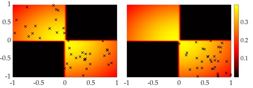
or because almost all trajectories in the dataset minimize or maximize some of the trajectory fea-
tures, accelerating and simplifying learning under the linear reward assumption. See Appendix G.2
for details about the trajectory features and how we generated the trajectory dataset.
We further analyze the querying methods in
this multimodal setting under the log-likelihood
metric in Fig. 4. Information gain significantly
outperforms random querying and volume re-
moval in both experiments with respect to the
AUC log-likelihood (p < 0.005). With respect
to the final log-likelihood, information gain re-
duces the amount of required data in LunarLan-
der by about 35% compared to random query-
ing and about 60% to volume removal. Sim-
ilarly in the Fetch Robot, the improvement is
approximately 25% over both baselines.
Appendix J presents two additional experi-
ments: one which clearly shows the effective- Figure 4: Different querying methods are compared
ness of our approach for learning a mixture of with the (top) MSE and (bottom) log-likelihood metrics
more than two reward functions (specifically, (mean±se over 75 runs).
M = 5), and one which studies the robustness against misspecified M .
Information Gain Leads to Better Learning. Having seen the superior predictive performance of
the reward learned via information gain optimization, we next assess its performance in the actual
environment. As random querying outperforms volume removal in terms of log likelihood and MSE
as in Fig. 4, we compare the information gain with random querying.
For this, we run the multimodal reward learning with 75 pairs of randomly generated reward weights
(M = 2 and K = 6). For each of the 150 individual reward functions, we compute the learned
policy rewards. Fig. 5 shows the results. While the standard errors in the plots seem high, this
is mostly because optimal trajectories for different reward weights differ substantially in terms of
rewards, which causes an irreducible variance. However, since the underlying true rewards are the
same between the information gain and random querying methods, we ran the paired sample t-
test between the results and observed statistical significance (p < 0.05). This means although the
learned policy rewards between different runs differ substantially, the reward function learned via
the information gain method leads to better task performance compared to random querying.
6       User Studies
We now empirically analyze the performance
of our algorithm with two online user stud-
ies.2 We again used the LunarLander and Fetch
Robot environments. We provide a summary               Figure 5: Information gain and random querying meth-
and a video of the user studies and their re-          ods are compared with the learned policy rewards
sults at https://sites.google.com/view/                (mean±se over 75 runs which correspond to 150 ran-
multimodal-reward-learning/.                           domly generated reward weights) in LunarLander.

Experimental Setup. For LunarLander, subjects were presented with either of the following in-
structions at every ranking query: “Land softly on the landing pad” or “Stay in the air as long as
possible”. We randomized these instructions such that users get one of them with 0.6 and the other
with 0.4 probability. We kept the presented instructions hidden from the learning algorithms so that
they need to learn a multimodal reward without knowing which mode each ranking belongs to.
For the Fetch robot environment, we recorded the 351 trajectories on the real robot as short video
clips so that the experiment can be conducted online under the pandemic regulations. Human sub-
jects participated in the experiment as groups of two to test learning from multiple users. Each
participant was instructed that the robot needs to put the banana in one of the shelves and different
shelves have different conditions (the same as in our running example, see Fig. 1, Appendix I.1).
After emphasizing there is no one correct choice and it only depends on their preferences, we asked
each participant to indicate their preferences between the shelves on an online form. Afterwards,
    2
        We have IRB approval from a research compliance office under the protocol number IRB-52441.

                                                      7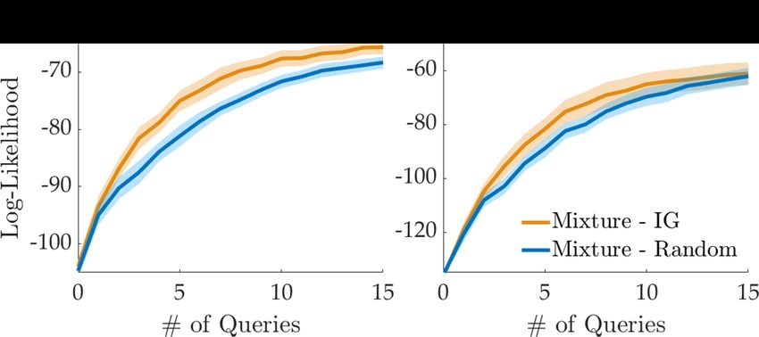
each group of two subjects responded to 30 ranking queries in total where each query consisted of 6
trajectories. We selected who responds to each query randomly, with probabilities 0.6 and 0.4.
Appendix I.2 presents details on the user interface used in our experiments.
Independent Variables. We varied the querying algorithm: active with information gain and ran-
dom querying. We excluded the volume removal method to reduce the experiment completion time
for the subjects, as it already performed worse than random querying in our simulations.
Procedure. We conducted the experiments as a within-subjects study. We recruited 24 participants
(ages 19 – 56; 9 female, 15 male) for LunarLander and 26 participants (ages 19 – 56; 11 female,
15 male) for the Fetch robot. Each subject in the LunarLander, and each group of two subjects in
the Fetch robot experiment responded to 40 ranking queries; 15 with each algorithm and 10 random
queries for evaluation at the end. The order of the first 30 queries was randomized to prevent bias.
Dependent Measures. Learning the multimodal reward functions via the 15 rankings collected by
each algorithm, we measured the log-likelihood of the final 10 rankings collected for evaluation.
Hypotheses. With LunarLander and Fetch robot, we test the following hypotheses respectively:
H1. Querying the participants, who are trying to teach two different tasks, actively with information
gain will lead to faster learning than random querying.
H2. While learning from two people with different preferences, active querying with information
gain will lead to faster learning than random querying.
Results. Figure 6 visualizes how log-likelihood
of the evaluation queries changes over the
course of learning by both algorithms. Active
querying with information gain leads to sig-
nificantly faster learning compared to random
querying in LunarLander. Indeed, the differ-
ence in AUC log-likelihood is statistically sig-
nificant (p < 0.05). Furthermore, the active
querying method enabled reaching the final per- Figure 6: User study results (mean±se over 24 users
formance of random querying after only 9 or 10 for LunarLander and 13 groups for Fetch Robot).
queries, for around a 35% reduction in the amount of data needed, supporting H1.
As the robot experiments have a an easier task with a small number of variables between the trajec-
tories, both querying methods converge to similar performances by the end of 15 queries. However,
active querying accelerates learning in the early stages—the difference in AUC log-likelihood is
again statistically significant (p < 0.05). Looking at the final performance with random querying,
improvement in data efficiency is about 10%, supporting H2.
7   Conclusion
Summary. This work presents a novel approach for learning multimodal reward functions. We for-
mulated the problem as a mixture learning problem solved using ranking queries that are answered
by experts. We further developed an active querying method that maximizes information gain to
improve the quality of ranking queries made to the experts. The results suggest our model learns
multimodal reward functions, with data efficiency improved by our new active querying method.
Limitations and Future Work. Our model for learning multimodal rewards requires knowing
the number of different modes (experts or tasks) M in advance. This might be difficult in some
settings. For example, when several experts belonging to different clusters, e.g., timid and aggressive
drivers, provide data, it might be difficult to know the number of clusters in advance. However, a
simple approach that fits the multimodal reward under various M could reveal the true number of
underlying modes. Another challenge is that learning a mixture reward model may contribute to
the reward ambiguity problem in inverse reinforcement learning: each individual reward may have
its own ambiguity. Future work should investigate the practical implications of this. In addition,
theoretical results assert, to guarantee the reliable learning of a multimodal reward with M modes,
ranking queries should consist of K queries such that M ≤ ⌊ K−2     2 ⌋!. While this is manageable by
multiple pairwise comparisons for each query or an iterative process where the expert selects the
top item, it might consume too much time for large M . Thus, an interesting future direction is to
investigate how to incorporate multiple forms of expert feedback, e.g., demonstrations in addition to
rankings, to pretrain and reduce the required interaction time with humans.

                                                  8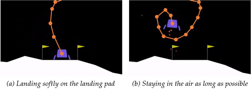
Acknowledgments
The authors would like to acknowledge funding by NSF grants #1849952 and #1941722, FLI grant
RFP2-000, and DARPA.
References
 [1] B. D. Ziebart, A. L. Maas, J. A. Bagnell, and A. K. Dey. Maximum entropy inverse reinforcement
     learning. In Aaai, volume 8, pages 1433–1438, 2008.
 [2] Z. Cao and D. Sadigh. Learning from imperfect demonstrations with varying dynamics. IEEE Robotics
     and Automation Letters, 2021.
 [3] D. H. Grollman and A. Billard. Donut as i do: Learning from failed demonstrations. In ICRA, 2011.
 [4] Y.-H. Wu, N. Charoenphakdee, H. Bao, V. Tangkaratt, and M. Sugiyama. Imitation learning from imper-
     fect demonstration. In Proceedings of the 36th International Conference on Machine Learning, volume 97
     of Proceedings of Machine Learning Research, pages 6818–6827. PMLR, June 2019.
 [5] E. Bıyık, D. P. Losey, M. Palan, N. C. Landolfi, G. Shevchuk, and D. Sadigh. Learning reward functions
     from diverse sources of human feedback: Optimally integrating demonstrations and preferences. The
     International Journal of Robotics Research (IJRR), 2021.
 [6] E. Biyik, N. Huynh, M. J. Kochenderfer, and D. Sadigh. Active preference-based gaussian process re-
     gression for reward learning. In Proceedings of Robotics: Science and Systems (RSS), July 2020.
 [7] A. Bajcsy, D. P. Losey, M. K. O’Malley, and A. D. Dragan. Learning from physical human corrections,
     one feature at a time. In Proceedings of the 2018 ACM/IEEE International Conference on Human-Robot
     Interaction, pages 141–149, 2018.
 [8] M. Li, A. Canberk, D. P. Losey, and D. Sadigh. Learning human objectives from sequences of physical
     corrections. In International Conference on Robotics and Automation (ICRA), 5 2021.
 [9] D. Brown, W. Goo, P. Nagarajan, and S. Niekum. Extrapolating beyond suboptimal demonstrations via
     inverse reinforcement learning from observations. In International Conference on Machine Learning,
     pages 783–792. PMLR, 2019.
[10] A. Shah and J. Shah. Interactive robot training for non-markov tasks. arXiv preprint arXiv:2003.02232,
     2020.
[11] K. Hausman, Y. Chebotar, S. Schaal, G. Sukhatme, and J. Lim. Multi-modal imitation learning from
     unstructured demonstrations using generative adversarial nets. In 31st Annual Conference on Neural
     Information Processing Systems (NIPS 2017), pages 1236–1246, 2018.
[12] C. Fei, B. Wang, Y. Zhuang, Z. Zhang, J. Hao, H. Zhang, X. Ji, and W. Liu. Triple-gail: A multi-
     modal imitation learning framework with generative adversarial nets. In Proceedings of the Twenty-Ninth
     International Joint Conference on Artificial Intelligence, IJCAI-20, pages 2929–2935, July 2020.
[13] M. Babes, V. N. Marivate, K. Subramanian, and M. L. Littman. Apprenticeship learning about multiple
     intentions. In ICML, 2011.
[14] G. Ramponi, A. Likmeta, A. M. Metelli, A. Tirinzoni, and M. Restelli. Truly batch model-free inverse
     reinforcement learning about multiple intentions. In International Conference on Artificial Intelligence
     and Statistics, pages 2359–2369. PMLR, 2020.
[15] B. Akgun, M. Cakmak, K. Jiang, and A. L. Thomaz. Keyframe-based learning from demonstration.
     International Journal of Social Robotics, 4(4):343–355, 2012.
[16] C. Basu, Q. Yang, D. Hungerman, M. Singhal, and A. D. Draqan. Do you want your autonomous car to
     drive like you? In 2017 12th ACM/IEEE International Conference on Human-Robot Interaction (HRI,
     pages 417–425, 2017.
[17] M. Kwon, E. Biyik, A. Talati, K. Bhasin, D. P. Losey, and D. Sadigh. When humans aren’t optimal:
     Robots that collaborate with risk-aware humans. In ACM/IEEE International Conference on Human-
     Robot Interaction (HRI), March 2020.
[18] C. Basu, M. Singhal, and A. D. Dragan. Learning from richer human guidance: Augmenting comparison-
     based learning with feature queries. In Proceedings of the 2018 ACM/IEEE International Conference on
     Human-Robot Interaction, pages 132–140, 2018.
[19] Z. Zhao, P. Piech, and L. Xia. Learning mixtures of plackett-luce models. In International Conference on
     Machine Learning, pages 2906–2914. PMLR, 2016.
[20] A. Y. Ng and S. Russell. Algorithms for inverse reinforcement learning. In in Proc. 17th International
     Conf. on Machine Learning, 2000.

                                                     9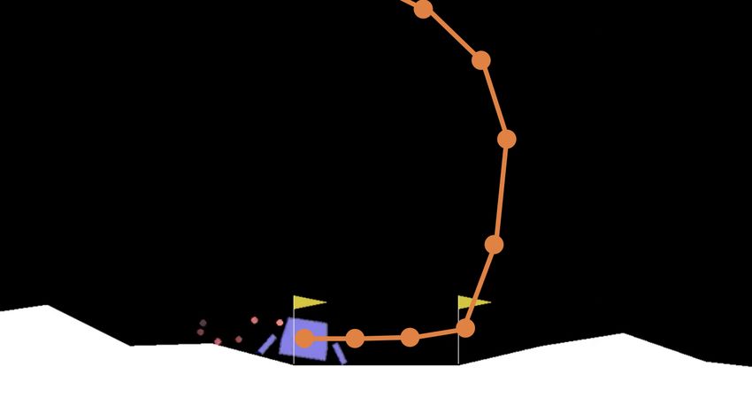
[21] P. Abbeel and A. Y. Ng. Apprenticeship learning via inverse reinforcement learning. In Proceedings of
     the twenty-first international conference on Machine learning, page 1, 2004.
[22] N. D. Ratliff, J. A. Bagnell, and M. A. Zinkevich. Maximum margin planning. In Proceedings of the 23rd
     international conference on Machine learning, pages 729–736, 2006.
[23] M. Cakmak, S. S. Srinivasa, M. K. Lee, J. Forlizzi, and S. Kiesler. Human preferences for robot-human
     hand-over configurations. In 2011 IEEE/RSJ International Conference on Intelligent Robots and Systems,
     pages 1986–1993, 2011.
[24] R. Akrour, M. Schoenauer, and M. Sebag. April: Active preference learning-based reinforcement learn-
     ing. In Joint European Conference on Machine Learning and Knowledge Discovery in Databases, pages
     116–131. Springer, 2012.
[25] D. Sadigh, A. D. Dragan, S. S. Sastry, and S. A. Seshia. Active preference-based learning of reward
     functions. In Proceedings of Robotics: Science and Systems (RSS), July 2017.
[26] P. F. Christiano, J. Leike, T. B. Brown, M. Martic, S. Legg, and D. Amodei. Deep reinforcement learning
     from human preferences. In NIPS, 2017.
[27] E. Biyik and D. Sadigh. Batch active preference-based learning of reward functions. In Proceedings of the
     2nd Conference on Robot Learning (CoRL), volume 87 of Proceedings of Machine Learning Research,
     pages 519–528. PMLR, October 2018.
[28] N. Wilde, D. Kulić, and S. L. Smith. Active preference learning using maximum regret. In 2020 IEEE/RSJ
     International Conference on Intelligent Robots and Systems (IROS), pages 10952–10959, 2020.
[29] E. Biyik, M. Palan, N. C. Landolfi, D. P. Losey, and D. Sadigh. Asking easy questions: A user-friendly
     approach to active reward learning. In Proceedings of the 3rd Conference on Robot Learning (CoRL),
     October 2019.
[30] M. Tucker, E. Novoseller, C. Kann, Y. Sui, Y. Yue, J. W. Burdick, and A. D. Ames. Preference-based
     learning for exoskeleton gait optimization. In 2020 IEEE International Conference on Robotics and
     Automation (ICRA), pages 2351–2357, 2020.
[31] K. Li, M. Tucker, E. Bıyık, E. Novoseller, J. W. Burdick, Y. Sui, D. Sadigh, Y. Yue, and A. D. Ames.
     Roial: Region of interest active learning for characterizing exoskeleton gait preference landscapes. arXiv
     preprint arXiv:2011.04812, 2020.
[32] L. Chen, H. Hassani, and A. Karbasi. Near-optimal active learning of halfspaces via query synthesis in
     the noisy setting. In Proceedings of the AAAI Conference on Artificial Intelligence, volume 31, 2017.
[33] R. Busa-Fekete and E. Hüllermeier. A survey of preference-based online learning with bandit algorithms.
     In International Conference on Algorithmic Learning Theory, pages 18–39. Springer, 2014.
[34] C. Wirth, R. Akrour, G. Neumann, J. Fürnkranz, et al. A survey of preference-based reinforcement
     learning methods. Journal of Machine Learning Research, 18(136):1–46, 2017.
[35] X. Chen, P. N. Bennett, K. Collins-Thompson, and E. Horvitz. Pairwise ranking aggregation in a crowd-
     sourced setting. In Proceedings of the sixth ACM international conference on Web search and data mining,
     pages 193–202, 2013.
[36] X. Chen, Y. Li, and J. Mao. A nearly instance optimal algorithm for top-k ranking under the multinomial
     logit model. In Proceedings of the Twenty-Ninth Annual ACM-SIAM Symposium on Discrete Algorithms,
     pages 2504–2522. SIAM, 2018.
[37] M. Ben-Akiva and S. R. Lerman. Discrete choice analysis: theory and application to travel demand.
     Transportation Studies, 2018.
[38] R. C. Wilson and A. G. Collins. Ten simple rules for the computational modeling of behavioral data.
     Elife, 8:e49547, 2019.
[39] E. Bıyık, D. A. Lazar, D. Sadigh, and R. Pedarsani. The green choice: Learning and influencing human
     decisions on shared roads. In 2019 IEEE 58th Conference on Decision and Control (CDC), pages 347–
     354, 2019.
[40] L. Maystre and M. Grossglauser. Fast and accurate inference of plackett-luce models. In Proceedings of
     the 28th International Conference on Neural Information Processing Systems-Volume 1, pages 172–180,
     2015.
[41] C. Archambeau and F. Caron. Plackett-luce regression: a new bayesian model for polychotomous data.
     In Proceedings of the Twenty-Eighth Conference on Uncertainty in Artificial Intelligence, pages 84–92,
     2012.
[42] T. Lu and C. Boutilier. Learning mallows models with pairwise preferences. In Proceedings of the 28th
     International Conference on International Conference on Machine Learning, pages 145–152, 2011.

                                                      10
[43] V. Vitelli, Ø. Sørensen, M. Crispino, A. Frigessi Di Rattalma, and E. Arjas. Probabilistic preference
learning with the mallows rank model. Journal of Machine Learning Research, 18(158):1–49, 2018.
[44] T. Lu and C. Boutilier. Effective sampling and learning for mallows models with pairwise-preference
data. Journal of Machine Learning Research, 15(117):3963–4009, 2014.
[45] R. Busa-Fekete, E. Hüllermeier, and B. Szörényi. Preference-based rank elicitation using statistical mod-
els: The case of mallows. In International Conference on Machine Learning, pages 1071–1079. PMLR,
2014.
[46] P. De Blasi, L. F. James, J. W. Lau, et al. Bayesian nonparametric estimation and consistency of mixed
multinomial logit choice models. Bernoulli, 16(3):679–704, 2010.
[47] F. Chierichetti, R. Kumar, and A. Tomkins. Learning a mixture of two multinomial logits. In International
Conference on Machine Learning, pages 961–969. PMLR, 2018.
[48] A. Liu and A. Moitra. Efficiently learning mixtures of mallows models. In 2018 IEEE 59th Annual
Symposium on Foundations of Computer Science (FOCS), pages 627–638, 2018.
[49] J. Morton and M. J. Kochenderfer. Simultaneous policy learning and latent state inference for imitat-
ing driver behavior. In 2017 IEEE 20th International Conference on Intelligent Transportation Systems
(ITSC), pages 1–6, 2017.
[50] C. Basu, E. Biyik, Z. He, M. Singhal, and D. Sadigh. Active learning of reward dynamics from hierarchi-
cal queries. In Proceedings of the IEEE/RSJ International Conference on Intelligent Robots and Systems,
2019.
[51] Z. Cao, E. Biyik, W. Z. Wang, A. Raventos, A. Gaidon, G. Rosman, and D. Sadigh. Reinforcement
learning based control of imitative policies for near-accident driving. In Proceedings of Robotics: Science
and Systems (RSS), July 2020.
[52] A. H. Qureshi, J. J. Johnson, Y. Qin, T. Henderson, B. Boots, and M. C. Yip. Composing task-agnostic
policies with deep reinforcement learning. In International Conference on Learning Representations,
2019.
[53] R. D. Luce. Individual choice behavior: A theoretical analysis. Courier Corporation, 2012.
[54] N. Ailon. An active learning algorithm for ranking from pairwise preferences with an almost optimal
query complexity. Journal of Machine Learning Research, 13(1), 2012.
[55] D. Bertsimas, J. Tsitsiklis, et al. Simulated annealing. Statistical science, 8(1):10–15, 1993.
[56] D. Golovin, A. Krause, and D. Ray. Near-optimal bayesian active learning with noisy observations. In
Proceedings of the 23rd International Conference on Neural Information Processing Systems-Volume 1,
pages 766–774, 2010.
[57] N. Houlsby, F. Huszár, Z. Ghahramani, and M. Lengyel. Bayesian active learning for classification and
preference learning. arXiv preprint arXiv:1112.5745, 2011.
[58] A. X. Zheng, I. Rish, and A. Beygelzimer. Efficient test selection in active diagnosis via entropy approx-
imation. In Proceedings of the Twenty-First Conference on Uncertainty in Artificial Intelligence, pages
675–682, 2005.
[59] G. Brockman, V. Cheung, L. Pettersson, J. Schneider, J. Schulman, J. Tang, and W. Zaremba. Openai
gym. arXiv preprint arXiv:1606.01540, 2016.
[60] M. Wise, M. Ferguson, D. King, E. Diehr, and D. Dymesich. Fetch and freight: Standard platforms for
service robot applications. In Workshop on autonomous mobile service robots, 2016.
[61] V. Mnih, K. Kavukcuoglu, D. Silver, A. Graves, I. Antonoglou, D. Wierstra, and M. Riedmiller. Playing
atari with deep reinforcement learning. arXiv preprint arXiv:1312.5602, 2013.
[62] S. Chib and E. Greenberg. Understanding the metropolis-hastings algorithm. The american statistician,
49(4):327–335, 1995.
[63] D. Golovin and A. Krause. Adaptive submodularity: Theory and applications in active learning and
stochastic optimization. Journal of Artificial Intelligence Research, 42:427–486, 2011.
11In the appendix, we provide additional details on the derivations of our methods and analysis, in ad-
dition to methodological details omitted from the main paper. In Appendix A, we directly derive the
formulas necessary for our querying via information gain optimization approach. Appendices B to D
present details on our main approach in Algorithm 1. Appendix E provides the arguments needed
to justify the claims of Section 4.4. Finally, Appendices F to I present details on our experimental
setups, while Appendix J presents a compelling additional synthetic data experiment demonstrating
learning a reward function mixture with five modes.
A Information Gain Derivation
We present the derivation of the formula for computing the maximum information gain query Q∗ .
′ ′
Assume at a fixed timestep t we have made past query observations D = {Q(t ) , x(t ) }t−1
t′ =1 . The
desired query is then
Q∗ = arg max I(Q; Θ | D), (6)
Q
where I(·; ·) denotes mutual information. Equivalently, denoting conditional entropy with H[· | ·],
we note [︂ ]︂ [︃ [︂ ]︂]︃
M M
I(Q; Θ | D) = H {αm , ωm }m=1 | D − E H {αm , ωm }m=1 | Q, X = x, D ,
P (X|Q,D)
which allows us to write the optimization in[︃ Eq. (6) equivalently as
[︂ ]︂]︃
M
Q∗ = arg min E H {α m , ω }
m m=1 | Q, X = x, D .
Q P (X|Q,D)
We further simplify this minimization objective by denoting the joint distribution over x and θ =
M
{αm , ωm }m=1 conditioned on Q and D as P (X, Θ | Q, D) and expanding the entropy term:
Pr [X = x | Q, D]
Q∗ = arg min E log
Q P (X,Θ|Q,D) Pr[X = x | Q, θ]
Eθ′ ∼Θ|D Pr [X = x | Q, θ′ ]
= arg min E log . (see 4)
Q P (X,Θ|Q,D) Pr[X = x | Q, θ]
B Metropolis-Hastings
B.1 Approach
To sample from Pr(Θ | D) using Eq. (3), we
use the Metropolis-Hastings algorithm [62], run-
ning N chains simultaneously for HM H itera-
tions. To avoid autocorrelation between sam-
ples, unlike in conventional Metropolis-Hastings
we only use the last state in each chain as a sam-
ple. In contrast, for conventional Metropolis-
Hastings, multiple samples would be drawn Figure 7: Multi-chain Metropolis-Hastings sampling
from a single chain at set intervals after a short (left) gives more representative samples from the dis-
burn-in period. As we see in Fig. 7, for our mul- tribution compared to the single-chain variant (right).
timodal Plackett-Luce posteriors, performing multi-chain Metropolis-Hastings yields posterior sam-
ples that are far more evenly distributed across different posterior modes. Thus, to achieve well-
distributed posterior samples, we set our effective burn-in period to be HM H − 1, taking only the
last sample from each chain.
M M
For two states in the chain Θ = {αm , ωm }m=1 and Θ′ = {αm
′
, ωm ′
}m=1 , our proposal distribution
is then
M
∏︂
g(Θ′ | Θ) = φ(ωm − ωm ′
),
m=1
where φ is the pdf of the diagonal Gaussian N (0, σM H I).
12B.2 Multimodal Metropolis-Hastings Demonstration
The posterior distribution in the figure is that of a 2-mode Plackett-Luce mixture with fixed uniform
mixing coefficients and 1-D weights conditioned on the observations 50 ≻ −50 and −50 ≻ 50. The
single-chain algorithm ran for 2000 steps with a burn-in period of 200 steps after which every 18th
sample was selected, while the multi-chain algorithm used 100 chains for 20 iterations each, taking
only the last sample from each chain.
C Simulated Annealing
For our simulated annealing, we run NSA chains in parallel for HSA iterations each, returning the
best query Q found across each run. We define the transition proposal distribution g(Q′ | Q) to
be a positive constant if Q′ and Q differ by one trajectory and 0 otherwise. We run with a starting
0
temperature of TSA , cooling by a factor of γSA with each subsequent iteration past the first.
D Hyperparameters
We use the hyperparameters in Table 1 for the simulated annealing and Metropolis-Hastings algo-
rithms, whose details are provided in Appendix B and Appendix C, respectively.
Table 1: Hyperparameters
Constant Value
N 100
HM H 200
σM H 0.15
NSA 10
HSA 30
0
TSA 10
γSA 0.9
E Proofs and Analysis
E.1 Proof of Corollary 1.1
⌊︁ 1.1.⌋︁ A mixture of M Plackett-Luce models with query size K is generically identifiable
Corollary
if M ≤ K−22 !.
Suppose we have such a mixture of M Plackett-Luce models that is not identifiable. Then, there
must exist two distinct sets of parameters Θ1 and Θ2 such that for every query Q, the induced
ranking distributions X1 and X2 respectively are identical. But since Θ1 and Θ2 are distinct, there
is either (1) two mixing coefficients in Θ1 and Θ2 that disagree or (2) two items ξ1 and ξ2 that
have a different difference in rewards across Θ1 and Θ2 under one of the reward functions. Let Q̄
with corresponding ranking distribution X̄ be an arbitrary query in case (1) and an arbitrary query
containing ξ1 and ξ2 in case (2). Note that X̄ is the marginal distribution of the overall Plackett-Luce
distribution, which by construction is a mixture of M Plackett-Luce models with parameters Θ1 and
Θ2 , restricted to the items in Q̄. But now there are two distinct sets of parameters representing the
distribution over the full ranking of Q since we know Θ1 and Θ2 differ on the restricted set of items
Ξ′ = Q (either because they have differing mixing coefficients or because their induced rewards on
Ξ′ are not a within a constant additive factor of each other since ξ1 and ξ2 are in Ξ′ ). But we know
|Ξ′ | = |Q| = K, so this finding contradicts the fact that X̄ must be identifiable by Theorem 1. We
conclude every mixture of M Plackett-Luce models is identifiable subject to the query size bounds
in the statement of this corollary.
E.2 Justification for Remark 1
Remark 1. Greedy selection of queries maximizing information gain in Eq. (4) is not necessarily
within a constant factor of optimality.
Here, we define the optimal adaptive set of queries D to be the one which, in expectation, mini-
mizes the uncertainty over model parameters H[Θ | D]. It is a well-known result that for adaptive
submodular functions, greedy optimization yields results that are within a constant factor 1 − 1e
(︁ )︁
of optimality [63]. While our mutual information objective in Eq. (4) is adaptive submodular in the
non-adaptive setting (where all queries Q are selected before observing their results), in our adap-
13tive setting these guarantees no longer hold (conditional entropy is only submodular with respect to
conditioned variables if those variables are unobserved).
F Baselines
F.1 Random
We benchmark against a random agent, wherein at each step the query selected by the agent is a
collection of K random items without replacement. We also use the random querying method for
comparing the multimodal reward learning with the existing approaches that assume a unimodal
reward (e.g. [5]), as it does not introduce any bias in the query selection.
F.2 Volume Removal
Volume removal seeks to maximize the difference between the prior distribution over model param-
eters and the unnormalized posterior. Volume removal notably fails to be optimal in domains where
there are similar trajectories [29]. In these settings, querying sets of trajectories with similar features
removes a large amount of volume from the unnormalized posterior (since the robot is highly un-
certain about their relative quality), yet yields little information about the model parameters (since
the human also has high uncertainty). Information gain approaches such as our method are better
able to generate trajectories to query for which the robot has high uncertainty while the human has
enough certainty to yield useful information for the robot.
G Trajectory Generation
G.1 LunarLander Trajectories
We designed 8 trajectory features based on: absolute heading angle accumulated over trajectory,
final distance to the landing pad, total amount of rotation, path length, task completion (or failure)
time, final vertical velocity, whether the lander landed on the landing pad without its body touching
the ground, and original environment reward from OpenAI Gym. Using these features, we randomly
generated 10 distinct reward functions based on the linear reward model and trained a DQN policy
[61] for each reward. Finally, we generated 100 trajectories by following each of these 10 policies in
the environment to obtain 1000 trajectories in total. We used these trajectories as our dataset for the
ranking queries. Fig. 8 presents an example trajectory with extracted scaled and centered features.
Feature Value
Mean angle 2.27683634
Total angle −0.20375356
Distance to Goal 5.41860642
Total rotation 0.25948072
Path length 3.71660086
Final vertical velocity −0.57097337
Crash time 1.11112885
Score −0.15500268
Figure 8: Sample LunarLander trajectory (left) with extracted features (right).
G.2 Fetch Trajectories
To design our 351 trajectories, we varied the target shelf (3 variations), the movement speed (3),
the grasp point on the banana (3) and where in the shelf it is placed (13). We then designed 12
trajectory features based on these varied parameters and appended another binary feature which
indicates whether any object dropped from the shelves on that trajectory.
Specifically, for τ a trajectory, let {︂
xi = 1 i is the target shelf ,
0 otherwise
14ygrasp , yheight , ywidth , yspeed specify the grasp position and speed, and ysuccess specify whether the robot
did not drop any objects from (︁ the shelves. Our featurization is then
Φ(τ ) = x1 , x2 , x3 , yspeed , yspeed (1 − yspeed ), ygrasp ,
ygrasp (1 − ygrasp ), yheight , yheight (1 − yheight ),
ywidth , ywidth (1 − ywidth ), 1 − (ygrasp − ywidth )2 , ysuccess .
)︁
Fig. 9 presents a sample Fetch trajectory with its featurization.
Feature Value
x1 1.0000
x2 0.0000
x3 0.0000
yspeed 0.5000
yspeed (1 − yspeed ) 0.2500
ygrasp 1.0000
ygrasp (1 − ygrasp ) 0.0000
yheight 0.7500
yheight (1 − yheight ) 0.1875
ywidth 0.2500
ywidth (1 − ywidth ) 0.1875
1 − (ygrasp − ywidth )2 0.4375
ysuccess 1.0000
Figure 9: Sample Fetch trajectory (left) with extracted features (right).
H Metrics
H.1 MSE
Our metric is
M
∑︂
∗
MMSE = ∥ωm ˆ︁m ∥22
−ω (7)
m=1
M M
where Θ∗ = {αm ∗
, ωm∗
}m=1 and Θ
ˆ︁ = {ˆ︁ ˆ︁m }m=1 and the learned reward weights of the ex-
αm , ω
perts are matched with the true weights using the Hungarian algorithm. When the learning model
assumes a unimodal reward function, as in our simulations for Fig. 3, we compute the MSE metric
∑︁M ∗
as m=1 ∥ωm − ω̂∥22 .
H.2 Log-Likelihood
Formally, we define the log-likelihood metric
[︁ as ]︁
MLL = EQ∼Q Ex∼P (X|Q) log Pr(x | Q, D) (8)
for Q the uniform distribution across all possible queries and P (x | Q) the distribution over the
human’s response to query Q (as in Eq. (2)). We can compute the inner term
Pr(x | Q, D) = EΘ|D [Pr(x | Q, Θ)]
using Metropolis-Hastings as in Section 4.3 to sample from the posterior Pr(Θ | D) and computing
the inner term with Eq. (2).
H.3 Learned Policy Rewards
Similar to the MSE metric, we match the rewards learned via DQN [61] with the true rewards using
the Hungarian algorithm.
I Experimental Setup
I.1 Shelf Descriptions
A picture of each shelf accompanied the following descriptions.
15You can also read