Link Prediction Approach to Recommender Systems
←
→
Page content transcription
If your browser does not render page correctly, please read the page content below
Noname manuscript No.
                                          (will be inserted by the editor)

                                         Link Prediction Approach to Recommender Systems

                                         T. Jaya Lakshmi · S. Durga Bhavani

                                         the date of receipt and acceptance should be inserted later
arXiv:2102.09185v1 [cs.IR] 18 Feb 2021

                                         Abstract The problem of recommender system is very popular with myriad available
                                         solutions. A novel approach that uses the link prediction problem in social networks
                                         has been proposed in the literature that model the typical user-item information as
                                         a bipartite network in which link prediction would actually mean recommending an
                                         item to a user. The standard recommender system methods suffer from the problems
                                         of sparsity and scalability. Since link prediction measures involve computations per-
                                         taining to small neighborhoods in the network, this approach would lead to a scalable
                                         solution to recommendation. One of the issues in this conversion is that link pre-
                                         diction problem is modelled as a binary classification task whereas the problem of
                                         recommender systems is solved as a regression task in which the rating of the link
                                         is to be predicted. We overcome this issue by predicting top k links as recommenda-
                                         tions with high ratings without predicting the actual rating. Our work extends similar
                                         approaches in the literature by focusing on exploiting the probabilistic measures for
                                         link prediction. Moreover, in the proposed approach, prediction measures that utilize
                                         temporal information available on the links prove to be more effective in improving
                                         the accuracy of prediction. This approach is evaluated on the benchmark ’Movielens’
                                         dataset. We show that the usage of temporal probabilistic measures helps in improv-
                                         ing the quality of recommendations. Temporal random-walk based measure T_Flow
                                         improves recommendation accuracy by 4% and Temporal cooccurrence probability
                                         measure improves prediction accuracy by 10% over item-based collaborative filtering
                                         method in terms of AUROC score.

                                         T. Jaya Lakshmi
                                         School of Engineering and Applied Sciences
                                         SRM University - Andhra Pradesh, India.
                                         E-mail: jaya.phd.hcu@gmail.com
                                         S. Durga Bhavani
                                         School of Computer and Information Sciences
                                         University of Hyderabad
                                         Hyderabad, India
                                         E-mail: sdbcs@uohyd.ernet.in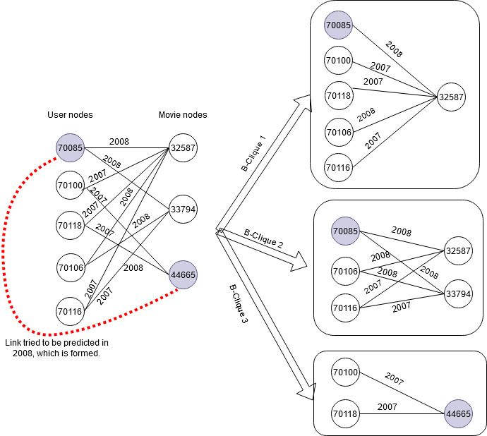
2                                                          T. Jaya Lakshmi, S. Durga Bhavani

1 Introduction

Many e-commerce websites provide a wide range of products to the users. The users
commonly have different needs and tastes based on which they buy the products. Pro-
viding the most appropriate products to the users make the buying process efficient
and improves the user satisfaction. The enhanced user satisfaction keeps the user
loyal to the website and improves the sales and thus profits to the retailers. Therefore,
more retailers start recommending the products to the users which needs efficient
analysis of user interests in products. E-commerce leaders like Amazon and Netflix
use recommender systems to recommend products to the users. The standard recom-
mendation algorithms like content-based filtering and collaborative filtering, model
the ratings given by users to items as a matrix and predict the ratings of the customers
to unrated items based on user/item similarity.
    Recommender systems recommend items to users. Items include products and
services such as movies, music, books, web pages, news, jokes and restaurants. The
recommendation process utilizes data including user demographics, product descrip-
tions and the previous actions of users on items like buying, rating, and watching. The
information can be acquired explicitly by collecting ratings given by users on items
or implicitly by monitoring user’s behavior such as songs listened in music web-
sites, news/movies watched in news/movies websites, items bought in e-commerce
websites or books read in book-listing websites in the past. Usage of intelligent rec-
ommendation systems improved the revenue of Amazon by 35%, caused a business
growth of 24% for BestBuy, increased 75% of views on Netflix and 60% views on
YouTube. [7]. Therefore, building a personalized recommendation system has a pro-
found significance not only in commercial arena, but also in the fields like health care,
news, food, academia and so many. Each domain needs to consider different features.
    Recommender system is a typical application of link prediction in heterogeneous
networks. Link Prediction problem infers future links in a network represented as
graph where nodes are users and edges denote interactions between users. In the
context of recommender systems, the nodes may be of two types: items and users. A
transaction of a user buying an item can be shown as an edge from user node to item
node. Recommendation problem can be viewed as a task of selecting unobserved
links for each user node, and thus can be modeled as a link prediction problem.
    In this work, we have applied various link prediction measures on the bipartite
network in the context of recommender systems and verified the efficacy of those
measures. We have chosen a medium sized dataset of MovieLens1M for experimen-
tation. The contributions made in this paper are

    – Evaluated the efficacy of base line link prediction measures to the recommenda-
      tion task.
    – Extended existing probabilistic measures called co-occurrence probability mea-
      sure and temporal co-occurrence probability measure to make it suitable for rec-
      ommendation problem.
Link Prediction Approach to Recommender Systems 3
item1 item2 item3 item4
5 2 User 1
4 4 2 User 2
R=
4 1 User 3
2 2 User 4
Fig. 1: Example rating matrix denoting rating given by users to 4 products.
Fig. 2: An example of user-item Bipartite Network with edges denoting rating given by user on item.
2 Problem Statement
Schafer et al [36] define the problem of recommender systems as follows:
Given a set of users U = {u1 , u2 , . . . um }, and items I = {I1 , I2 , . . . , In } and the
ratings R representing the ratings given by user ui to item I j , the task of recommender
systems is to recommend a new item I j to a user ui which the user ui did not buy.
For example, consider the matrix given in Fig.1, where rows correspond to the
users and the columns denote products. The matrix entry Ri j represents the rankings
given by user ui on item I j . The main task of the recommender systems is to predict
the unrated entries in the rating matrix.
Recommender systems are natural examples of weighted bipartite networks. A
Bipartite network contains exactly two types of nodes and single type of edges
existing between different types of nodes. Bipartite network is defined as G = (V1 ∪
V2 , E), where V1 and V2 are sets of two types of nodes, E represents the set of
edges between nodes of type V1 and V2 . Fig.2 depicts a sample scenario of users
buying items in e-commerce sites such as Amazon, modeled as a bipartite network.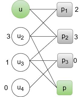
4                                                        T. Jaya Lakshmi, S. Durga Bhavani

                    Fig. 3: Taxonomy of recommender systems

3 Related Literature

The papers on recommender system in the literature are discussed from algorithmic
as well as domain perspective in the next two sections. Fig. 3 gives a taxonomy of the
literature.

3.1 Domain Perspective

Product recommendation is the mostly explored domain. E-commerce sites like Ama-
zon, Flipkart, Ebay etc use various collaborative filtering techniques for recommend-
ing products to their customers. Video recommendations like movies, TV shows and
web series are increasing exponentially by companies like Netflix, YouTube. Netflix
has launched a competition with 1Million dollars prize money for improving 10% of
RMSE in the movie recommendation, by releasing a 100 million customer ratings [5].
A news recommendation system has been implemented in [27] using google news,
by constructing a Bayesian network for identifying the user interests and then apply-
ing content based as well as collaborative filtering and hybrid techniques. Research
article recommendation, food recommendation and health recommendation are other
domains among many.
    Valdez et al. integrate recommender systems into individual medical records to
help patients improve their autonomy. The authors have collected health related infor-
mation from the patients’ records and have performed text processing for extracting
features and evaluated using metrics available in Information Extraction domain [38].
    All these domains need different pre-processing techniques, algorithms, and eval-
uation metrics.
Link Prediction Approach to Recommender Systems 5
3.2 Algorithmic perspective
Recommender systems is seeing an explosive growth in the literature with many
novel algorithms being proposed almost every day. Content-based recommendation,
Collaborative Filtering (CF) and Hybrid approach are some of the popular approaches
that solve the problem of recommender systems. Context aware recommender sys-
tems predict recommendations based on user context. Graph based recommender sys-
tems is main focus of this work. In graph based recommender system, the purchases
are modeled as bipartite graph and various graph traversal techniques are applied to
generate a set of co-purchased items/users.
3.2.1 Content-based recommendation
Content-based recommendation uses item descriptions and constructs user profiles
which contain the information about user preferences [32]. These user preferences
may include a genre, director and actor for a movie, an author for book etc. The rec-
ommendation of an item to the user is then based on the similarity between the item
description and the user profile. This method has the benefit of recommending items
to users that have never been rated by them [29]. Content-based recommendation sys-
tems require complete descriptions of items and detailed user profiles. This is one of
the main limitations of such systems [29].
Content-based recommender systems are divided into three general approaches:
Explicit, Implicit and Model-based. In explicit content based methods, profile in-
formation of the users is collected through questionnaires that ask questions about
their preferences for the items. Implicit methods build the user profiles implicitly
by searching for similarities in liked and disliked item descriptions by the user. The
third class of methods, viz., model-based methods construct user profiles based on a
learning method, using item descriptions as input features to be given to a supervised
learning algorithm, and producing user ratings of items as output.
The item descriptions are often textual information contained in documents, web
sites and news messages. User profiles are modeled as weighted vectors of these
item descriptions. The advantage of this method is the ability to recommend newly
introduced items to users [29]. Content-based recommendation systems require the
complete descriptions of items and detailed user profiles. This is the main limitation
of such systems. Privacy issues such as users dislike to share their preferences with
others is another limitation of content-based systems.
3.2.2 Collaborative filtering
Collaborative filtering systems, however, do not require such difficult to come by,
well-structured item descriptions. Instead, they are based on users’ preferences for
items, which can carry a more general meaning than is contained in an item descrip-
tion. Indeed, viewers generally select a film to watch based upon more criteria other
than only its genre, director or actors.
Collaborative filtering (CF) techniques depend only on the user’s past behavior
and provide personalized recommendation of items to users [26]. CF techniques take6 T. Jaya Lakshmi, S. Durga Bhavani
a rating matrix as input where the rows of the matrix correspond to users, the columns
correspond to items and the cells correspond to the rating given by the user to the
item [20]. The rating by a user to an item represents the degree of preference of
the user towards the item. The major advantage of the CF methods is they are domain
independent. CF methods are classified into Model-based CF [18] and Memory-based
CF. Model based techniques model ratings by describing both items and users on
some factors induced by matrix factorization strategies. Data sparsity is a serious
problem of CF methods.
Model based approaches such as dimensionality reduction techniques, Principal
Component Analysis (PCA), Singular Value Decomposition (SVD) are some of the
popular techniques that address the problem of sparsity. However, when certain users
or items are ignored, useful information for recommendations may be lost causing
reduction in the quality of recommendation [33]. The limitation of collaborative fil-
tering systems is the cold start problem. i.e., these methods can not recommend new
items to the existing users as there is no past buying history for the item. Similarly, it
is difficult to recommend items to a new user without knowing the user’s interests in
the form of ratings.
Memory based methods compute a set of nearest neighbors for users as well as
items using similarity measures like Pearson coefficient, cosine distance and Manhat-
tan distance. Memory based CF techniques are further classified into user based and
item based [37].
User-based CF [12] User based methods compute the similarity between the users
based on their ratings on items [13]. This creates a notion of user neighborhoods.
These methods associate a set of nearest neighbors with each user and then predict
the user’s rating for unrated items utilizing the information of the neighbor’s rating
for that item.
Item-based CF [34]: Similarly, item neighborhood depicts the number of users who
rate the same items [35]. The item rating for a given user can then be predicted based
upon the ratings given in their user neighborhood and the item neighborhood. These
methods associate an item with a set of similar neighbors, and then predict the user’s
rating for an item using the ratings given by the user for the nearest neighbors of the
target item.
3.2.3 Hybrid approach
Hybrid approach uses both types of information, collaborative and content based.
Content boosted CF algorithm [28], uses the item profile information to recommend
the items to new users.
3.2.4 Context aware recommendation system
Context aware recommendation system is able to label each user action with an ap-
propriate context and effectively tailor the system output to the user in that given
context [3]. In [17], the authors proposed a recommendation of an activity to a socialLink Prediction Approach to Recommender Systems 7
network user based on demographic information. Kefalas et al. have represented their
data as a k-partite network modeled as a tensor and proposed novel algorithms. In the
same way, in [4], a citation recommendation is made to researchers also considering
tags and time. Standard recommender system algorithms cannot address these issues.
3.2.5 Graph based Recommender Systems
Li et al. map transactions to a bipartite user–item interaction graph and thus con-
verting recommendation into a link prediction problem. They propose a kernel-based
recommendation approach which generate random walk between user–item pair and
define similarities between user–item pairs based on the random walks. Li et al. use a
kernel-based approach that indirectly examines customers and items related to user-
item pair to foresee the existence of an edge between them. The paper uses a set
of nodes representing two types of nodes users(U) and items(I) and edges denoting
transactions by the user regarding the items. The graph kernel is defined on the user-
item pairs context [22].
Zhang et al. propose a model for music recommendation [40]. The authors repre-
sent the recommendation data as a bipartite graph with user and item nodes and the
weight of the link is represented as a complex number depicting the dual preference
of users in the form of like and dislike and improve the similarity of the users.
In graph-based recommender system, the task of recommendation is equivalent
to predicting a link between user-item based on graphical analysis. Link prediction
in graphs is commonly a classification task, that predicts existence of a link in fu-
ture [23]. But the problem of recommender systems is modeled as a regression task,
which predicts the rating of a link. The predicted links with high ratings are gen-
erally recommended to users. The standard techniques of recommendation systems
take the ratings matrix as input and predicts the empty cells in the matrix. This ap-
proach severely suffer with the sparsity in the matrix. Ranking-oriented collaborative
filtering approach is more meaningful compared to the rating based approach be-
cause, the recommendation is a ranking task recommending top-k ranked items to
a user [9]. In some applications like recommending web pages, rating information
may not be available. Graph-based recommendation can efficiently utilize the hetero-
geneous information available in the networks by expanding the neighborhoods and
can compute the proximity between the users and items [37].
A probabilistic measure for predicting future links in bipartite networks is given
in [14]. Several link prediction measures in various kinds of networks have been
summarized in [19].
Our aim is to evaluate the efficacy of these measures in the context of recom-
mender systems by modeling them as bipartite graphs. In this paper, we have applied
various existing link prediction measures on bipartite graphs in order to build a rec-
ommender system. However, the link prediction approach does not give the actual
rating, but gives the top k-item recommendations for a user. For experimentation, we
have chosen the bench-mark ’Movielens’ dataset. Next section gives an overview of
application of link prediction measures on bipartite graphs.8 T. Jaya Lakshmi, S. Durga Bhavani
4 Link Prediction in bipartite graph
Graph-based recommendation algorithms compute recommendations on a bipartite
graph where nodes of the graph represent users and items and an edge forms between
a user node and an item node when the user buys the item. Once the transactions
are modeled as a graph, all the standard link prediction methods defined in [23],[25]
can be applied directly on the graph to predict the future links [21]. All the measures
used in [23] are based on neighbors and paths. Especially, common neighbors, which
lie on paths of length two play an important role. All the measures are extended to
heterogeneous environment in [19] with a mention of bipartite networks as special
case.
We follow similar notation as in [19] in this paper, which is given below.
– (u, p) is a pair of user and product nodes without an edge between them.
– k represents hop-distance between two nodes and t denotes time.
– Γk (x) is the set of k-hop neighbors of node x. Γ1 (x) refers to the set of all nodes
connected by an edge of any type to x generally written as Γ (x).
– Γ (u) ∩ Γ (p) denotes the set of common neighbors between node u and p. In
bipartite graph, this set is empty.
– Γk (u) ∩ Γk (p) contains all the common neighbors within k-hop distance between
nodes u and p. In bipartite graph, k needs to be even to start and end path between
same type of nodes and odd if path starts and ends between nodes of different
types. As recommender system tries to recommend items to users, the odd length
paths are meaningful.
– Pk (u, p) denotes the set of paths connecting u and p by at most k edges.
4.1 Baseline link prediction measures in bipartite graph
In recommendation systems modeled as bipartite graph, the task is to recommend
products to users. The product nodes and user nodes are connected with odd length
paths. Even length paths connect the nodes of same type, which is not meaningful in
this scenario. Keeping this in mind, the baseline link prediction measures for bipartite
graphs are given below. We use suffix B with all link prediction measures to indicate
they are used in context of bipartite network.
– Common Neighbors (CN) : The common neighbor measure in bipartite graph is
given as follows:
CNB (u, p) = |Γ3 (u) ∩ Γ3 (p)| (1)
Jaccard Coefficient, AdamicAdar and Preferential Attachment measures are also
neighborhood-based defined in a similar way as follows.
– Jaccard Coefficient (JC) : Jaccard Coefficient is the normalized CN measure
|Γ3 (u) ∩ Γ3 (p)|
JCB (u, p) = (2)
|Γ3 (u) ∪ Γ3 (p)|Link Prediction Approach to Recommender Systems 9
– Adamic Adar (AA) : This measure gives importance to the common neighbors
with low degree. The following definition for bipartite networks has been hinted
at [10].
1
AAB (u, p) = ∑ (3)
z∈Γ (u)∩Γ (p)
log(|Γ3 (z)|)
3 3
– Preferential Attachment (PA) : This measure does not change in bipartite en-
vironment because the measure is concerned only about the degree of the node
whatever the type of the node may be.
PAB (u, p) = |Γ1 (u)| ∗ |Γ1 (p)| (4)
– Katz (KZ) : This measure is based on the total number of paths between u and p
bounded by a limit penalized by path length.
KZB (u, p) = ∑ β l |Pl (u, p)l | (5)
l
– Page Rank (PR) : This measure can be extended to heterogeneous network by
including the heterogeneous edges in the random-walk.
1−α PR(z)
PRB (u) = +α ∑ (6)
|E| |Γ
z∈Γ (u) 3
(z)|
3
where |E| is the total number of links in G.
– Rooted Page Rank (RPR) : In order to make the measure PR symmetric, Rooted
Page Rank is computed for an edge (u, p) as follows.
RPRB (u, p) = PR(u, p) + PR(p, u) (7)
– PropFlow (PF) : This is a random-walk beginning at node u and ending at p
within l steps. This random-walk from node u to p terminates either when it
reaches p or revisits any node. PFB (u, p) is the probability of information flow
from u to p based on random transmission along all paths defined recursively as
follows.
L
PFB (u, p) = ∑ ∑ ∑ PF(z1 , z2 ) (8)
l=2 p∈pathsl (u,p) ∀(z1 ,z2 )∈p
where
w(z1 , z2 )
PFB (z1 , z2 ) = PF(a, z1 ) ∗ (9)
∑ w(z1 , z)
z∈Γ (z1 )
with a as previous node of z1 in the random-walk, PF(a, z1 )=1 if a is the starting
node and pathsl (u, p) is the set of paths of length l between u and p. In bipartite
network, l is odd.10 T. Jaya Lakshmi, S. Durga Bhavani
L
PFB (u, p) = ∑ ∑ ∑ PFB (z1 , z2 ) (10)
l=2 p∈Pl (u,p) ∀(z1 ,z2 )∈p
where PFB (z1 , z2 ) is as defined in Eq.9.
4.2 Temporal measures for link prediction in bipartite graph
4.2.1 Time-Score(T SB )
We extend Time-Score measure proposed for homogeneous networks [31] to bipartite
environment as follows:
w(path) ∗ β r(path)
T SB (u, p) = ∑ (11)
path∈P (u,p)
|latest(path) − oldest(path)| + 1
3
where w(path) is equal to the harmonic mean of edge weights of edges in path, β
is a damping factor (0Link Prediction Approach to Recommender Systems 11
4.2.3 T_Flow(T FB )
T_Flow [30] is a random-walk based measure, which is an extension of PropFlow
measure defined in [25]. Munasinghe et.al [30] define T_Flow that computes the
information flow between a pair of nodes x and y through all random-walks starting
from node u to node p including link weights as well as activeness of links by giving
more weight to recently formed links recursively and take the summation.
We extend T_Flow measure to bipartite networks as follows:
l
T FB (u, p) = ∑ ∑ ∑ T FB (z1 , z2 ) ∗ (1 − α)r(path) (14)
i=2 path∈Pl (x,y) ∀e∈path
If (u, p) ∈ E, then T FB (u, p) is given by
w(u, path)
T FB (u, p) = T FB (a, u) ∗ ∗ (1 − α)r(path) (15)
∑ w(u, z)
z∈Γ (u)
where tu is the time stamp of the link when the random walk visits the node u and t p
is the time stamp of the link when the random walk visits node p.
4.3 Probabilistic measure for link prediction in bipartite graph
The Probabilistic Graphical Model (PGM) represents the structure of the graph in
a natural way by considering the nodes of graph as random variables and edges as
dependencies between them. By representing a graph as a PGM, the problem of link
prediction, which is calculation of the probability of link formation between two
nodes u, p is translated to computing the joint probability of the random variables
U, P.
Recommender systems represented as bipartite networks are large in size. There-
fore, finding the joint probabilities of link formation is intractable. But the links in the
graphs are also sparse, with nodes generally directly connected to only a few other
nodes. For example, in the e-commerce sites, out of lakhs of items, a user buys only
a few items. This property allows the PGM distribution to be represented tractably.
The model of this framework is simple to understand. Inference between two random
variables is same as finding the joint probability between those two random variables
in PGM. Many algorithms are available for computation of joint probability between
variables, given evidence on others. These inference algorithms work directly on the
graph structure and are generally faster than computing the joint distribution explic-
itly. With all these advantages, link prediction in PGM is more effective.
In most of the cases, the pair-wise interactions of entities are available in the event
logs. For example, a user buying/rating three items say p1 , p2 and p3 is available in
the corresponding transaction database. In order to model the unknown distribution
of co-occurrence probabilities, events available in the event logs can be used as con-
straints to build a model for the unknown distribution. Probabilistic Graphical Models12 T. Jaya Lakshmi, S. Durga Bhavani
efficiently utilize this higher order topological information and thus are efficient in
link prediction task [39].
The probabilistic model helps in estimating the joint probability distribution over
the variables of the model [11]. That means, a probabilistic model represents the prob-
ability distribution over all possible deterministic states of the model. This facilitates
the inference of marginal probabilities of the individual variables of the model.
Wang et al. [39] are among first researchers who modeled the problem of link
prediction using MRFs. Kashima et al. [16] propose a probabilistic model of net-
work evolution and apply it for predicting future links. The authors show that by
intelligently selecting the parameters in an evolution model, the problem of network
evolution reduces to the problem of link prediction. Clauset et al. [8] propose a proba-
bilistic model based on hierarchical structure of the network. In hierarchical structure,
the vertices are divided into groups that further subdivide into groups of groups and
so on. The model infers hierarchical structure from network data and can be used for
prediction of missing links. The learning task uses the observed network data and
infers the most likely hierarchical structure through statistical inference.
The works of Kashima [16] and Clauset [8] are global models and are not scal-
able for large networks. The method of Wang et. al. [39] uses local probabilistic
information of graphs for link prediction and we adopt their method in our work. The
following section explains the algorithm for link prediction using MRF proposed by
Wang et al. [39]
5 Proposed approach: Link Prediction in bipartite networks induced as PGM
Wang et al. [39] propose a measure called Co-occurrence Probability (COP) to be
computed between a pair of nodes without an edge between them. The procedure for
computing COP has three steps. First step chooses a few set of nodes which may play
a significant role in future link formation. Second step computes a Markov Random
Field with the chosen nodes in the first step. Third step infers joint probability be-
tween the two nodes using the MRF constructed. The measure has been extended to
temporal networks in [15]. Heterogeneous version of the measure is defined in [14].
Though Hetero-COP has been defined in [14], the algorithm has to be re-worked for
the bipartite context. In this paper, we have extended COP measure to bipartite envi-
ronment, named it as B-COP of a missing link (u, p) in the lines of COP, which is
given in Algorithm 1. The extended computation procedure for bipartite networks is
given in subsequent sections.Link Prediction Approach to Recommender Systems 13
Algorithm 1 B-COP measure for Link Prediction in bipartite graphs
Input: G = (V, E), where
V = {V1 ∪V2 } is the set of two types of nodes,
E is the set of links from nodes of V1 to V2 .
Output: B-COP(u, p) where (u, p) is a missing link.
Step 1: Extract B-cliques from G, from the event logs using Algorithm 3. Call it BCliq.
Step 2: Compute BCNS, the central neighborhood set of (u, p) using the Algorithm 2.
Step 3: Extract B-cliques formed with the nodes in BCNS and compute clique potentials. This forms
the local MRF with the nodes in BCNS.
Step 4: Return B-COP(u, p) which is the joint probability of link (u, p) using junction tree algorithm.
A clique in bipartite graphs can be considered as complete bipartite sub-
graph. A sample B-clique is shown in Fig.4.
Fig. 4: An example B-clique.
5.1 Computation of Central Neighborhood Set in Bipartite graph(BCNS)
BCNS(u, p) is computed using a breadth first search based algorithm on bipartite
graph as follows: All paths between u and p are obtained using breadth first search
(BFS) algorithm. Then, the frequency score of each path is computed by summing
the occurrence count of nodes on the path. Occurrence count of a node is the number
of times the node appears in all paths. The paths are now ordered in the increasing
order of length with equal paths being ordered in decreasing order of frequency score.
The size of the central neighborhood set is further restricted by considering only top
k nodes. The procedure of computing BCNS(u, p) is described in the Algorithm 2.
The procedure of computation of BCNS for a toy example given in Fig.5 is shown
in Table 1.14 T. Jaya Lakshmi, S. Durga Bhavani
Algorithm 2 Bipartite Central Neighborhood Set(G, u, p, l, maxSize)
Input: G: a graph; u: starting node; p: ending node; l:maximum path length; maxSize:Central Neighbor-
hood Set size threshold
Output: BCNS, Bipartite Central Neighborhood Set between u and p;
Step 1: Compute paths of length ≤ l between u and p.
Step 2: Find occurrence count Ok of each node k in paths between u and p.
Step 3: Compute f requency-score Fp , of each path p as follows:
Fp = ∑k∈p Ok
f requency-score of a path is the sum of the occurrence counts of all nodes along the paths.
Step 4: Sort the paths in increasing order of path length and then in decreasing order of f requency-
score. Let the ranked list of paths be P.
Step 5:
while size(BCNS) ≤ maxSize do
Add nodes of path p ∈ P to BCNS
end while
return BCNS
path(p) frequency-score(Fp )
u − p2 − u2 − p O p2 + O u2 = 6
u − p1 − u2 − p O p1 + O u2 = 5
u − p2 − u3 − p O p2 + O u3 = 4
u − p1 − u2 − p2 − u3 − p O p1 + Ou2 + O p2 + Ou3 = 9
Table 1: All paths between nodes u and p in Fig.5
and their frequency scores.
Fig. 5: A toy example for illustrating
computation of BCNS between nodes u
and p. Node weights are the occurrence
counts.
Table 1 shows all paths sorted in the increasing order of path length and fre-
quency score, between the nodes u and p of the graph shown in Fig.5 along with
their f requency-scores. One can observe that all these paths are of odd length. For
the bipartite graph in Fig.5, BCNS(u, p) = {u, p2 , u2 , p1 , p}, if maxSize is taken as 5.
5.2 Construction of local MRF
After computing the BCNS, the B-cliques containing only nodes of BCNS are ex-
tracted. This forms the clique graph of local MRF. MRF construction needs compu-
tation of clique potentials. The clique potential table of a B-clique is computed using
the NDI.
In most of the cases, the information of homogeneous cliques containing all nodes
of same type are available in the event logs. For example, in coauthorship networks,
the group of authors who publish a paper together forms a homogeneous clique of
author nodes and an author who publishes a paper in a conference forms a heteroge-
neous edge between the author node and conference node. But in the case of recom-Link Prediction Approach to Recommender Systems 15
mender systems, user cliques and item cliques are not readily available in the event
logs. We propose an algorithm for extracting B-cliques shown in Algorithm 3. Since
the number of users is huge in comparison to the set of items which is a much smaller
set, the extraction of B-cliques can start from the item cliques.
Algorithm 3 Extraction of B-Cliques from user-item bipartite graph
Input: G = (V, E) where V = U ∪ I, U is set of user nodes and I is the set of item nodes and E ⊆ UXI
represents weighted edges.
Output: Bcliq, set of maximal B-cliques of G.
Step 1: Extract the set of all item cliques, Item_Cliq as follows:
Item_Cliq = φ
for each user u ∈ U do
Iu = φ
for each i ∈ I and (u, i) ∈ E do
Iu = Iu ∪ {i}
end for // Iu is formed by taking all the items to which u gives a rating.
Item_Cliq = Item_Cliq ∪ Iu
end for
Step 2: Extract the set of all user cliques, User_Cliq as follows:
User_Cliq = φ
for each item i ∈ do
Ui = φ
for each u ∈ U and (u, i) ∈ E do
Ui = Ui ∪ {u}
end for // Ui contains all users that have rated item i.
User_Cliq = User_Cliq ∪Ui
end for
Step 3:
for each item i in I do
J←I
for each user v in Ui do
J ← J ∩ Iv
end for \
// J = Iv //
v∈Ui
Bcliqi = J ∪Ui
Bcliq = ∪i Bcliqi
end for
return Bcliq
The B-clique extraction algorithm first extracts all homogeneous cliques of items
Icliq and users Ucliq. A homogeneous user clique is formed with all the users who
rate/buy the same item. Similarly, a homogeneous clique of items is formed with all
the items a user rate/buy. To extract a B-clique, first consider an item i. For each user
v who have rated i, compute the common items rated by user v. The union of Ui along
with all the common items rated by Ui forms a B-clique. The process of extracting
B-cliques for toy example in Fig.6 is illustrated below:16 T. Jaya Lakshmi, S. Durga Bhavani
U={u1 , u2 , u3 , u4 , u5 } I={i1 , i2 , i3 , i4 , i5 }
Item cliques :
Item clique corresponding to user u1 = {i1 , i2 }
Item clique corresponding to user u2 = {i1 , i2 }
Item clique corresponding to user u3 = {i2 , i3 , i4 , i5 }
Item clique corresponding to user u4 = {13 , i4 , i5 }
Item clique corresponding to user u5 = {13 , i4 , i5 }
User cliques :
User clique corresponding to item i1 = {u1 , u2 }
User clique corresponding to item i2 = {u1 , u2 , u3 }
User clique corresponding to item i3 = {u3 , u4 , u5 }
User clique corresponding to item i4 = {u3 , u4 , u5 }
User clique corresponding to item i5 = {u3 , u4 , u5 }
The the extraction of B-cliques from the above homoge-
neous cliques is shown in Fig.7.
Fig. 6: User-Item
bipartite graphLink Prediction Approach to Recommender Systems 17
Fig. 7: Illustration of extracting B-cliques from User-Item event logs18 T. Jaya Lakshmi, S. Durga Bhavani
5.3 Computation of B-COP score
Once the local MRF of a pair of nodes u and p is constructed, the B-COP score
between the nodes is obtained using junction tree inference algorithm. Note that B-
COP score for a link u - p cannot be computed if u and p are in disjoint cliques as
there exists no path connecting these cliques.
The experimental evaluation of proposed approach is given in next section.
6 Experimental Evaluation
The experimentation is carried out on a benchmark MovieLens recommender system
whose details are given below.
6.1 Dataset
This data set used for experimental evaluation contains more than ten million rat-
ings given by 71,567 users on 10,681 movies of the online movie recommender ser-
vice MovieLens [1]. In the graph recommendation systems, movies are considered as
nodes and items are users and rating given by users to the movies are considered as
the weights on links. In MovieLens dataset, the train-test splits are given in [1]. The
users who have rated at least 20 movies have been chosen randomly to be included
in this dataset. The benchmark data set [2] is given with 80% - 20% split with 80%
given as training set and test set containing 20%. The training and test sets are formed
by splitting the ratings data such that, for every user, 80% of his/her ratings is taken
in training and the rest are taken in the test set. In this experimentation, 5 fold cross
validation is used. All the 5 sets of training and test datasets are made available at
[2]. The evaluation metrics used for recommender systems are given in the following
section.
6.2 Evaluation Metrics
Evaluation metrics in recommender systems can be classified as
– Accuracy measures: Mean Absolute Error (MAE), Root of Mean Square Error
(RMSE), Normalized Mean Average Error (NMAE).
– Set recommendation metrics : Precision, Recall and Area Under Receiver Oper-
ating Characteristic (AUROC), Area Under Precision-recall curve (AUPR)
– Rank recommendation metrics: Half-life, discounted cumulative gain and Rank-
score
Most of the measures listed above, use rating to calculate the error and
hence are not applicable in our context. We use AUROC, AUPR are used for evalu-
ating performance.Link Prediction Approach to Recommender Systems 19
Rank-score Rank-score metric measures the ability of a recommendation algorithm
to produce a ranked list of recommended items. The recommender system method is
efficient, if the ranking given by the method matches with the user’s order of buying
the items in the recommended list. Rank-score is defined as follows : For a user u,
the list of items i recommended to u, that is predicted by the algorithm is captured by
rankscore p
1
rankscoremax = |T | j−1
∑ j=1 2 α
1
rankscore p = rank( j)−1
∑ j∈T 2 α
rankscore p
Rankscore =
rankscoremax
where rank( j) is the rank given by the recommender algorithm to item j. T is the
set of items of interest and α is ranking half-life, an exponential reduction factor and
can be any numeric.
6.3 Results and Discussion
The prediction scores of all baseline link prediction measures are computed using
the tool LPMade [24], with default parameters. In the computation of T SB , LSB and
T PI, the damping factor β is taken as 0.5. The decay factor α is considered as 0.1
in computation of T FB . In TCOP, maximum path length of 10 is taken for comput-
ing BCNS. The accuracy of all these link prediction measures is compared with the
standard User-based and Item-based collaborative filtering (CF) methods. Pearson
correlation coefficient is used to find the similar users in User-based CF and cosine
similarity is used for finding item similarity in Item-based CF.
The results obtained for AUROC, AUPR and Rank-score for MovieLens dataset
are given in Table.2.
First observation in this experimentation is that some of the link prediction mea-
sures like Katz, PropFlow could produce better recommendation compared to Item-
based CF. The usage of temporal measures seem to help in improving the quality of
recommendations. The time of formation of link or the time of rating given by a user
to movie plays crucial role, as the user’s preferences change over time. The temporal
measures TS, LS, TF and TCOP assign more weight to the recent ratings. Therefore,
temporal measures performed better than all the other measures including User-based
CF and Item-based CF. Fig.8 depicts a situation where non-temporal measures predict
a link between the nodes 1 and 1080 and temporal measures predict correctly that the
link won’t be formed. This is clearly evident from the fact that B − Cliq1 is formed
with very old links formed in the year 1996 compared to the prediction year 2008.
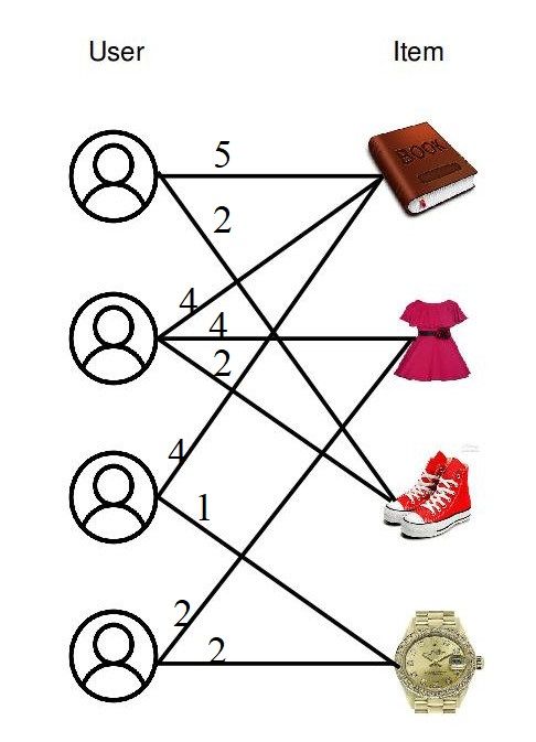
Fig.9 depicts the situation where the temporal links predict correctly. TCOP outper-
formed all the other link prediction measures and the user-based and item-based col-
laborative filtering methods. The recommendation performance is improved by 6% in
terms of AUROC over TF and nearly 10% over CF methods. It can be observed from20 T. Jaya Lakshmi, S. Durga Bhavani
Table 2: Performance of LP measures for recommending movies to users in
MovieLens Bipartite Network
LP measure Rank-score AUROC AUPR
Non-temporal LP measures
CNB 2.0501 0.5123 0.0092
JCB 1.3615 0.4956 0.0085
AAB 1.7819 0.5749 0.0153
PAB 2.6804 0.6832 0.0251
KZB 3.2546 0.6635 0.0193
PFB 3.2990 0.6846 0.0286
COPB 3.6661 0.7231 0.0613
Temporal LP measures
T SB 4.0015 0.7016 0.0365
LSB 5.2134 0.7340 0.0861
T FB 5.3684 0.7532 0.0960
TCOPB 8.6304 0.8165 0.2351
Classical Collaborative Filtering methods
User-based CF 3.9942 0.6925 0.0415
Item-based CF 3.0274 0.7136 0.0491
Fig. 8: A snapshot from movielens dataset where the link predicted is not formed.
Table.2 that the AUPR score also have shown great improvement from 0.0960(of TF)
to 0.2351. Similar trend is observed for the evaluation measure of Rank-score. All
the temporal measures perform better than User-based CF and Item-based CF. TCOP
is rated as highest by Rank-score.Link Prediction Approach to Recommender Systems 21 Fig. 9: A snapshot from movielens dataset where the link predicted is formed. 7 Conclusion In this paper, the recommender systems problem is solved using link prediction ap- proach. Link prediction approach is scalable as it is based on local neighborhood of the large sparse graph. The standard recommender systems approaches do not utilize the temporal information available on the link effectively. In this work, some exten- sions are proposed to existing temporal measures in bipartite graphs. One of the main contributions of this work is an algorithm for computing temporal cooccurrence prob- ability measure on bipartite graphs and its application to movie recommendation sys- tem. Temporal measures for link prediction such as Time score, Link Score, T_Flow and Temporal cooccurrence measure achieve improvement in recommendation qual- ity by utilizing this temporal information more efficiently. However, link prediction approach to solve recommender systems do not address the cold start problem. In future, we would like to work on predicting actual rating of the link.
22                                                                  T. Jaya Lakshmi, S. Durga Bhavani

References

 1. https://grouplens.org/datasets/, 2009.
 2. http://files.grouplens.org/datasets/movielens/ml-10m-README.html, 2009.
 3. Gediminas Adomavicius, Bamshad Mobasher, Francesco Ricci, and Alexander Tuzhilin. Context-
    aware recommender systems. AI Magazine, 32(3):67–80, 1 2011.
 4. Zafar Ali, Guilin Qi, Pavlos Kefalas, Waheed Ahmad Abro, and Bahadar Ali. A graph-based taxon-
    omy of citation recommendation models. Artificial Intelligence Review, pages 1–44, 2020.
 5. Robert M Bell and Yehuda Koren. Lessons from the netflix prize challenge. Acm Sigkdd Explorations
    Newsletter, 9(2):75–79, 2007.
 6. Pankaj Choudhary, Nishchol Mishra, Sanjeev Sharma, and Ravindra Patel. Link score: A novel
    method for time aware link prediction in social network. ICDMW, 2013.
 7. Michael Chui. Artificial intelligence the next digital frontier? McKinsey and Company Global Insti-
    tute, 47:3–6, 2017.
 8. Aaron Clauset, Cristopher Moore, and Mark EJ Newman. Hierarchical structure and the prediction of
    missing links in networks. Nature, 453(7191):98, 2008.
 9. Paolo Cremonesi, Yehuda Koren, and Roberto Turrin. Performance of recommender algorithms on
    top-n recommendation tasks. In Proceedings of the Fourth ACM Conference on Recommender Sys-
    tems, RecSys ’10, pages 39–46. ACM, 2010.
10. Darcy A. Davis, Ryan Lichtenwalter, and Nitesh V. Chawla. Supervised methods for multi-relational
    link prediction. Social Network Analysis and Mining, 3(2):127–141, 2013.
11. Marek J. Druzdzel. Some properties of joint probability distributions. In Proceedings of the Tenth
    International Conference on Uncertainty in Artificial Intelligence, UAI’94, pages 187–194. Morgan
    Kaufmann Publishers Inc., 1994.
12. Zan Huang, Wingyan Chung, and Hsinchun Chen. A graph model for e-commerce recommender
    systems. J. Am. Soc. Inf. Sci. Technol., 55(3):259–274, 2004.
13. Zan Huang, Wingyan Chung, and Hsinchun Chen. A graph model for e-commerce recommender
    systems. Journal of the American Society for information science and technology, 55(3):259–274,
    2004.
14. T. Jaya Lakshmi and S. Durga Bhavani. Link prediction in temporal heterogeneous networks. In
    Intelligence and Security Informatics, pages 83–98. Springer International Publishing, 2017.
15. T. Jaya Lakshmi and S. Durga Bhavani. Temporal probabilistic measure for link prediction in collab-
    orative networks. Applied Intelligence, 47(1):83–95, Jul 2017.
16. H. Kashima, T. Kato, Y. Yamanishi, M. Sugiyama, and K. Tsuda. Link propagation: A fast semi-
    supervised learning algorithm for link prediction. In Proceedings of the 2009 SIAM International
    Conference on Data Mining, pages 1099–1110. Philadelphia, PA, USA, May 2009.
17. Pavlos Kefalas, Panagiotis Symeonidis, and Yannis Manolopoulos. A graph-based taxonomy of rec-
    ommendation algorithms and systems in lbsns. IEEE Transactions on Knowledge and Data Engi-
    neering, 28(3):604–622, 2015.
18. Yehuda Koren, Robert Bell, and Chris Volinsky. Matrix factorization techniques for recommender
    systems. Computer, 42(8):30–37, 2009.
19. T Jaya Lakshmi and S Durga Bhavani. Link prediction measures in various types of information
    networks: a review. In 2018 IEEE/ACM International Conference on Advances in Social Networks
    Analysis and Mining (ASONAM), pages 1160–1167. IEEE, 2018.
20. Jure Leskovec, Anand Rajaraman, and Jeffrey David Ullman. Recommendation Systems, page
    292–324. Cambridge University Press, 2 edition, 2014.
21. Jing Li, Lingling Zhang, Fan Meng, and Fenhua Li. Recommendation algorithm based on link predic-
    tion and domain knowledge in retail transactions. Procedia Computer Science, 31:875 – 881, 2014.
22. Xin Li and Hsinchun Chen. Recommendation as link prediction in bipartite graphs: A graph kernel-
    based machine learning approach. Decision Support Systems, 54(2):880–890, 2013.
23. David Liben-Nowell and Jon Kleinberg. The link-prediction problem for social networks. Journal of
    The American Society For Information Science and Technology, 58(7):1019–1031, 2007.
24. Ryan N. Lichtenwalter and Nitesh V. Chawla. Lpmade: Link prediction made easy. Journal of
    Machine Learning Research., 12:2489–2492, 2011.
25. Ryan N. Lichtenwalter, Jake T. Lussier, and Nitesh V. Chawla. New perspectives and methods in
    link prediction. In Proceedings of the 16th ACM SIGKDD international conference on Knowledge
    discovery and data mining, KDD’10, pages 243–252. ACM, 2010.
Link Prediction Approach to Recommender Systems 23
26. Greg Linden, Brent Smith, and Jeremy York. Amazon. com recommendations: Item-to-item collabo-
rative filtering. IEEE Internet computing, 7(1):76–80, 2003.
27. Jiahui Liu, Peter Dolan, and Elin Rønby Pedersen. Personalized news recommendation based on
click behavior. In Proceedings of the 15th international conference on Intelligent user interfaces,
pages 31–40, 2010.
28. Prem Melville, Raymod J. Mooney, and Ramadass Nagarajan. Content-boosted collaborative filtering
for improved recommendations. In Eighteenth National Conference on Artificial Intelligence, pages
187–192. American Association for Artificial Intelligence, 2002.
29. Raymond J. Mooney and Loriene Roy. Content-based book recommending using learning for text
categorization. In Proceedings of the Fifth ACM Conference on Digital Libraries, DL ’00, pages
195–204. ACM, 2000.
30. Lankeshwara Munasinghe. Time-aware methods for link prediction in social networks. PhD Thesis,
The Graduate University for Advanced Studies, 2013.
31. Lankeshwara Munasinghe and Ryutaro Ichise. Time aware index for link prediction in social net-
works. In DaWaK, volume 6862 of Lecture Notes in Computer Science, pages 342–353. Springer,
2011.
32. Michael J. Pazzani and Daniel Billsus. The adaptive web. chapter Content-based Recommendation
Systems, pages 325–341. Springer-Verlag, 2007.
33. Badrul Sarwar, George Karypis, Joseph Konstan, and John Riedl. Analysis of recommendation algo-
rithms for e-commerce. In Proceedings of the 2Nd ACM Conference on Electronic Commerce, EC
’00, pages 158–167. ACM, 2000.
34. Badrul Sarwar, George Karypis, Joseph Konstan, and John Riedl. Item-based collaborative filtering
recommendation algorithms. In Proceedings of the 10th International Conference on World Wide
Web, WWW ’01, pages 285–295. ACM, 2001.
35. Badrul Sarwar, George Karypis, Joseph Konstan, and John Riedl. Item-based collaborative filtering
recommendation algorithms. In Proceedings of the 10th international conference on World Wide Web,
pages 285–295, 2001.
36. J. Ben Schafer, Joseph A. Konstan, and John Riedl. E-commerce recommendation applications. Data
Mining and Knowledge Discovery, 5(1):115–153, 2001.
37. Bita Shams and Saman Haratizadeh. Graph-based collaborative ranking. Expert Syst. Appl., 67(C):59–
70, 2017.
38. André Calero Valdez, Martina Ziefle, Katrien Verbert, Alexander Felfernig, and Andreas Holzinger.
Recommender systems for health informatics: state-of-the-art and future perspectives. In Machine
Learning for Health Informatics, pages 391–414. Springer, 2016.
39. Chao Wang, Venu Satuluri, and Srinivasan Parthasarathy. Local probabilistic models for link predic-
tion. In Proceedings of Seventh IEEE International Conference on Data Mining, ICDM ’07, pages
322–331. IEEE Computer Society, 2007.
40. Lingling Zhang, Minghui Zhao, and Daozhen Zhao. Bipartite graph link prediction method with
homogeneous nodes similarity for music recommendation. Multimedia Tools and Applications, pages
1–19, 2020.You can also read