Localizing and Orienting Street Views Using Overhead Imagery - arXiv.org
←
→
Page content transcription
If your browser does not render page correctly, please read the page content below
Localizing and Orienting Street Views Using
                                                          Overhead Imagery

                                                                    Nam N. Vo and James Hays

                                                                   Georgia Institute of Technology
                                                                     {namvo,hays}@gatech.edu

                                               Abstract. In this paper we aim to determine the location and orienta-
                                               tion of a ground-level query image by matching to a reference database
                                               of overhead (e.g. satellite) images. For this task we collect a new dataset
arXiv:1608.00161v2 [cs.CV] 22 Mar 2017

                                               with one million pairs of street view and overhead images sampled from
                                               eleven U.S. cities. We explore several deep CNN architectures for cross-
                                               domain matching – Classification, Hybrid, Siamese, and Triplet net-
                                               works. Classification and Hybrid architectures are accurate but slow since
                                               they allow only partial feature precomputation. We propose a new loss
                                               function which significantly improves the accuracy of Siamese and Triplet
                                               embedding networks while maintaining their applicability to large-scale
                                               retrieval tasks like image geolocalization. This image matching task is
                                               challenging not just because of the dramatic viewpoint difference be-
                                               tween ground-level and overhead imagery but because the orientation
                                               (i.e. azimuth) of the street views is unknown making correspondence even
                                               more difficult. We examine several mechanisms to match in spite of this
                                               – training for rotation invariance, sampling possible rotations at query
                                               time, and explicitly predicting relative rotation of ground and overhead
                                               images with our deep networks. It turns out that explicit orientation
                                               supervision also improves location prediction accuracy. Our best per-
                                               forming architectures are roughly 2.5 times as accurate as the commonly
                                               used Siamese network baseline.

                                               Keywords: Image Geolocalization, Image Matching, Deep Learning,
                                               Siamese Network, Triplet Network

                                         1   Introduction
                                         In this work we propose deep learning approaches to the problem of ground to
                                         overhead image matching. Such approaches enable large scale image geolocaliza-
                                         tion techniques to use widely-available overhead/satellite imagery to estimate
                                         the location of ground level photos. This is in contrast to typical image geolocal-
                                         ization which relies on matching “ground-to-ground” using a reference database
                                         of geotagged photographs. It is comparatively easy (for humans and machines)
                                         to determine if two ground level photographs depict the same location, but the
                                         world is very non-uniformly sampled by tourists and street-view vehicles. On the
                                         other hand, overhead imagery densely covers the Earth thanks to satellites and
                                         other aerial surveys. Because of this widespread coverage, matching ground-level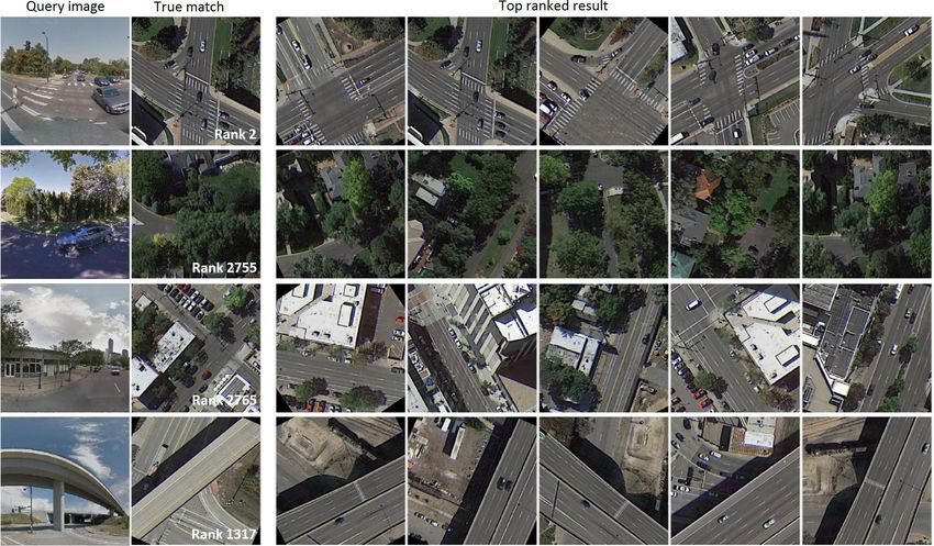
2      Nam N. Vo and James Hays

photos to overhead imagery has become an attractive geolocalization approach
[19]. However, it is a very challenging task (even for humans) because of the huge
viewpoint variation and often lighting and seasonal variations, too. In this paper
we try to learn how to match urban and suburban images from street-view to
overhead-view imagery at fine-scale. As shown in Figure 1, once the matching is
done, the results can be ranked to generate a location estimate for a ground-level
query.
    To address cross-view geolocalization, the community has recently found
deep learning techniques to outperform hand-crafted features [20, 34]. These ap-
proaches adopt architectures from the similar task of face verification [7, 29].
The method is as follows: a CNN, more specifically a Siamese architecture net-
work [5, 7], is used to learn a common low dimensional feature representation for
both ground level and aerial image, where they can be compared to determine
a matching score. While being superior to non-deep approaches (or pre-trained
deep features), we show there is significant room for improvement.

               Fig. 1. Street-view to overhead-view image matching

    To that end we study different deep learning approaches for matching/verification
and ranking/retrieval tasks. We develop better loss functions using the novel
distance based logistic (DBL) layer. To further improve the performance, we
show that good representations can be learned by incorporating rotational in-
variance (RI) and orientation regression (OR) during training. Experiments are
performed on a new large scale dataset which will be published to encourage
future research. We believe the findings here generalize to similar matching and
ranking problems.

1.1   Related work
Image geolocalization uses recognition techniques from computer vision to
estimate the location (at city, region, or global scale) of ordinary ground level
photographs. Early work by Hays and Efros [12] studied the feasibility of this
task by leveraging millions GPS-tagged images from the Internet. In [37], image
localization is done efficiently by building a dataset of Google street-view images
from which SIFT features are extracted, indexed and used for localization of
a query image by voting. Lin et al. [19] propose the first ground-to-overhead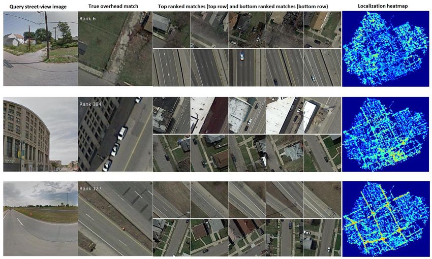
Localizing and Orienting Street Views Using Overhead Imagery            3

geolocalization method. No attempt is made to learn a common feature space or
match directly across views. Instead, ground-to-ground matching to a reference
database of ground-overhead view pairs is used to predict the overhead features
of a ground-level query. Bansal et al. [3] match street-level images to aerial images
by proposing a feature which encodes facade structure self-similarity. Shan et al.
[27] propose a fully automated system that registers ground-based multi-view
Stereo models to aerial imagery using traditional multi-view and Structure from
Motion technique.
    Deep learning has been successfully applied to a wide range of computer
vision tasks such as recognition of objects [17], places [39], faces [29]. Most re-
cently, “PlaNet” [33] made use of a large amount of geo-tagged images, quantized
the gps-coordinate into a number of regions and trained a CNN to classify an
image’s location into one of those regions. More relevant to this work is deep
learning applications in cross-view images matching [20, 34]. The most similar
published work to ours is Lin et al. [20] which uses a Siamese network to learn a
common deep representation of street-view images and 45 degree aerial or bird’s
eye images. This representation is shown to be better than hand-crafted or off-
the-shelf CNN features for matching buildings’ facades from different angles. In
[34], Workman et al. show that by learning different CNNs for different scales
(i.e. using aerial images at certain scales), geolocalization can be done at the
local or continental level. Interestingly, they also showed that by fixing the rep-
resentation of ground-level image, which is 205 categories scores learned from
the Places database [39], the CNN will learn the same category scores for aerial
images. Most recently, Altwaijry et al. [2] use a deep attentive architecture to
match aerial images across wide baselines.

2    Dataset of street view and overhead image pairs

Fig. 2. On the left: visualization of the positions of all Miami’s panorama images that
we randomly collect for further processing. On the right: examples of produced street-
view and overhead pairs.

    We study the problem of matching street-view image to overhead images
for the application of image geolocalization. To that end, we collect a large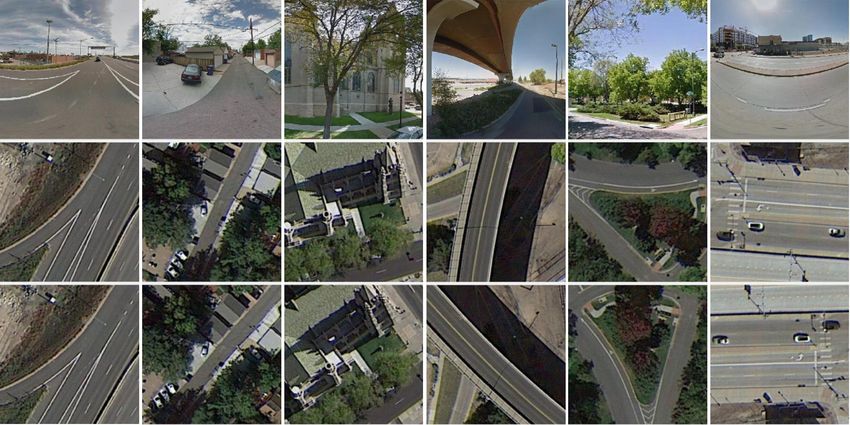
4       Nam N. Vo and James Hays

scale dataset of street-view and overhead images. More specifically, we randomly
queried street-view panorama images from Google Map of the US. For each
panorama, we randomly made several crops and for each crop we queried Google
Map for the overhead image at the finest scale, resulting in an aligned pair
of street-view and overhead images. Note that we want to localize the scene
depicted in the image and not necessarily the camera. This is possible since
Google panorama images come with geo-tags and depth estimates. We performed
this data collection procedure on 11 different cities in the US and produced more
than 1 million pairs of images. Some example matches in Miami are shown in
Figure 2. We make this dataset available to the public.
    Some similar attempts to collect a dataset for cross-view images matching
task are [20, 34], but neither are publicly available. We expect that the result and
analysis here can be easily generalized across other datasets (or other applica-
tions like recognizing face or object instead of scene). While the technical aspects
are similar, there will be qualitative differences: when training on [20], the net-
work learns to match the facade which is visible from both views. On [34], the
network learns to match similar categories of scenes or land cover types. And on
our dataset, the network learns to recognize different fine-grained street scenes.

3     Cross-view matching and ranking with CNN

Before considering the ranking/retrieval task, we start with the matching/verification
task formalized as following: during training phase, matched pairs of street-view
and overhead images are provided as positive examples (negative examples can
be easily generated by pairing up non-matched images) to learn a model. During
testing, given a pair of images, the learned model is applied to classify if the pair
is a match or not.
    We use deep CNNs which have been shown to perform better than traditional
hand-crafted features, especially for problems with significant training data avail-
able. We study 2 categories of CNNs (Figure 3): the classification network for
recognizing matches and the representation learning networks for embedding
cross-view images into the same feature space. Note that the first category is
not practical for the large-scale retrieval application and is used as a loose upper
bound for comparison.
    The second category includes the popular Siamese-like network and the
triplet network. We introduce another version of Siamese and triplet networks
that use the distance based logistic layer, a novel loss function. For completeness
we also include the Siamese-classification hybrid network (which will belong to
the first category). In this section we will experiment with 6 networks in total.

3.1   Classification CNN for image matching

Since our task is basically classification, the first network we experiment with
is AlexNet[17], originally demonstrated for object classification (Figure 3(a)). It
has 5 convolutional layers, followed by 3 fully-connected layers and a soft-max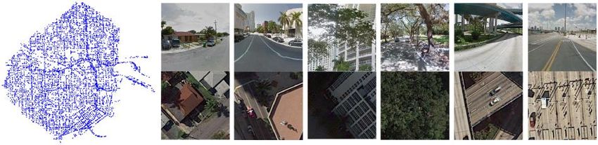
Localizing and Orienting Street Views Using Overhead Imagery            5

Fig. 3. Different CNN architectures: on the left is the first category: the classifica-
tion network and the Siamese-classification hybrid network, on the right is the second
category: the Siamese network and the triplet network

layer for classification. We make several modifications: (1) the input will be a
6-channel image, a concatenation of a street-view image and an overhead image,
while the original AlexNet only takes 1-image input , (2) we double the number
of filters in the first convolutional layer, (3) we remove the division of filters into
2 groups (this was done originally because of GPU memory limitation) and (4)
the softmax layer produces 2 outputs instead of 1000 because our task is binary
classification. Similar architectures have been used for comparing image patches
[36].
    Training the CNN is done by minimizing this loss function:

                      L(A, B, l) = LogLossSof tM ax(f (I), l)                      (1)

where A and B are the 2 input images, l ∈ {0, 1} is the label indicating if it’s
a match, I = concatenation(A, B) and f (.) is the AlexNet that outputs class
scores.

3.2   Siamese-like CNN for learning image features

The Siamese-like network, shown in Figure 3(b), has been used for cross-view
image matching [20, 34] and retrieval [30, 4]. It consists of 2 separate CNNs.
Each subnetwork takes 1 image as input and output a feature vector. Formally,
given 2 images A and B, we can apply the learned network to produce the
representation f(A) and f(B) that can be used for matching. This is done by
computing the distance between these 2 vectors and classifying it as a match if
the distance is small enough. During training, the contrastive loss is used:

                   L(A, B, l) = l ∗ D + (1 − l) ∗ max(0, m − D)                    (2)

   where D is the squared distance between f(A) and f(B), and m is the margin
parameter that omits the penalization if the distance of non-matched pair is big
enough. This loss function encourages the two features to be similar if the images
are a match and separates them otherwise; this is visualized in Figure 4(left).
6       Nam N. Vo and James Hays

Fig. 4. Visualization of Siamese network training. We represent other instances
(matches and non-matches) relative to a fixed instance (called the anchor). Left:
with contrastive loss, matched instances keep being pulled closer, while non-matches
are pushed away until they are out of the margin boundary, Right: log-loss with
DBL: matched/nonmatched instances are pushed away from the “boundary” in the
inward/outward direction.

    In the original Siamese network [10], the subnetworks (f(A) and f(B)) have the
same architecture and share weights. In our implementation, each subnetwork
will be an AlexNet without weight sharing since the images are of different
domains: one is street view and the other is overhead.

3.3   Siamese-classification hybrid network

The hybrid network is similar to the Siamese in that the input images are pro-
cessed independently to produce output features and it is similar to the classifi-
cation network that the features are concatenated to jointly infer the matching
probability (Figure 3(c)). Similar architectures have been used for used for cross-
view matching and feature learning [36, 1, 11, 2].
    Formally let AlexNet (f ) is consist of 2 parts: the set of convolutional layers
(fconv ) and the set of fully-connected layers (ff c ), the loss function is:

                  L(A, B, l) = LogLossSof tM ax(ff c (Iconv ), l)                (3)

     Where Iconv = concatenation(fconv (A), fconv (B)). We expect this network
to approach the accuracy of the classification network, while being slightly more
efficient because intermediate features only need to be computed once per image.

3.4   Triplet network for learning image features

The fourth network that we call the triplet network or ranking network, shown in
Figure 3(c), is popular for image feature learning and retrieval [35, 31, 24, 32, 26,
25], though its effectiveness has not been explored in cross-view image matching.
More specifically it aims to learn a representation for ranking relevance between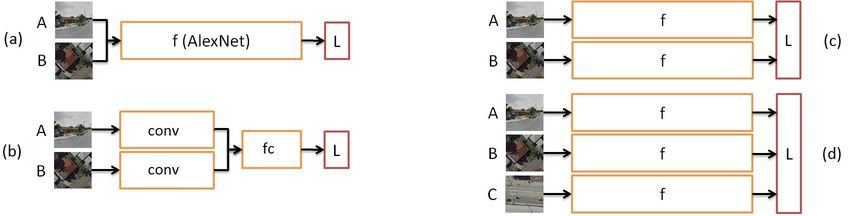
Localizing and Orienting Street Views Using Overhead Imagery         7

images. It consists of 3 separate CNNs instead of 2 in the Siamese network.
Formally, the network takes 3 images A, B and C as inputs, where (A,B) is a
match and (A,C) is not, and minimizes this hinge loss for triplet (which has been
explored before its application in deep learning [6, 22]):

                 L(A, B, C) = max(0, m + D(A, B) − D(A, C))                     (4)

    Where D is the squared distances between the features f(A), f(B), f(C), and m
is the margin parameter to omit the penalization if the gap between 2 distances
is big enough. This loss layer encourages the distance of the more relevant pair
to be smaller than the less relevant pair (Figure 5(left)).
    In the context of image matching, a pair of matched images (as the anchor
and the match), plus a random image (as the non-match) is used as training
example. With the learned representation, matching can be done by thresholding
just like the Siamese network case.

3.5   Learning image representations with distance-based logistic loss
Despite being intuitive to understand, common loss functions based on euclidean
distance might not be optimal for recognition. We instead advocate loss functions
similar to the standard softmax, log-loss.
    For the Siamese network, instead of the contrastive loss, we define the dis-
tance based logistic (DBL) layer for pairs of inputs as:

                                         1 + exp(−m)
                           p(A, B) =                                            (5)
                                       1 + exp(D − m)

This outputs a value between 0 and 1, as the probability of the match given
the squared distance. Then we can use the log-loss like the classification case for
optimization:
                       L(A, B, l) = LogLoss(p(A, B), l)                         (6)
   The behavior of this loss is visualized in Figure 4(right). Notice the difference
from the traditional contrastive loss.
   For the triplet network, we define the DBL for triple as following:
                                              1
                   p(A, B, C) =                                                 (7)
                                  1 + exp(D(A, B) − D(A, C))

This represents the probability that it’s a valid triple: B is more relevant to A
than C is to A (note that p(A, B, C) + p(A, C, B) = 1). Similarly the log-loss
function is used, so:

                 L(A, B, C) = log(1 + exp(D(A, B) − D(A, C)))                   (8)

    The behavior of this loss is visualized in Figure 5(right).
    With this novel layer, we obtain Siamese and triplet DBL-Net that allow us
to optimize for the recognition accuracy more directly. As with the original loss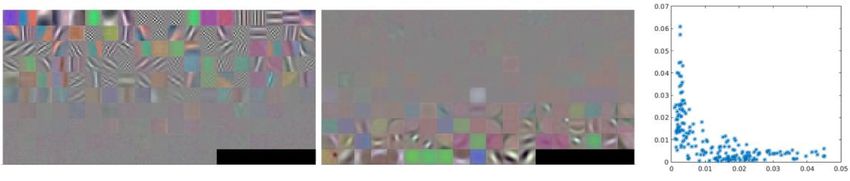
8       Nam N. Vo and James Hays

Fig. 5. Visualization of triplet network training. Each straight line originating from
the anchor represents a triple. Left: with triplet/ranking loss, instances are pulled and
pushed until the difference between the match distance and the non-match distance
is bigger than the threshold, Right: log loss with DBL for triple. Similar to the rank-
ing loss, but instead of relying on the threshold, the “force” depends on the current
performance and confidence of the network.

functions, the learned feature representation can be used for efficient matching
and ranking at test time (when the DBL layer is not involved).
    Implementation detail: we use m=10; and D(.) is squared Euclidean dis-
tance. We do not do feature normalization (L2) in all of our experiment; hence
the network can change the scale of the feature and the formulas here can be
applied directly. However if there’s normalization which basically predefined the
scale of the output feature (and therefore the distance between them), it’s best
to scale the feature by a suitable constant (for example 3) before applying the
DBL-log loss. Or equivalently change/validate the steepness and the midpoint
of the logistic curve (instead of using the standard logistic function form).

4    Learning to perform rotation invariant matching
As we are considering the task of fine-grained street view to overhead view
matching, not only spatial but also orientation alignment is important, i.e. ro-
tating the overhead image according to the street-view’s orientation instead of
keeping the overhead image north oriented.
    We aim to learn a rotation invariant (RI) representation of the overhead
images. Similarly, Ke at al [16] studied the problem of shape recognition without
explicit alignment. In [21], nearby filters are untied to potentially allow pooling
on output of different filters. This helps to learn complex representation without
big filters or increasing the number of filters; however that doesn’t result in an
explicit RI property like we desire. Deep symmetry network [9] is capable of
encoding such a property, though its advantage is not significant when training
data is sufficient for traditional CNN to learn that on its own. More relevant, [8]
uses data augmentation and concatenation of features from different viewpoints.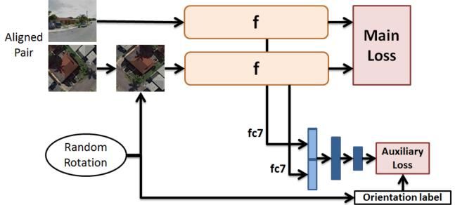
Localizing and Orienting Street Views Using Overhead Imagery           9

However our training data comes with orientation aligned images (though not
the test sets), which can potentially provide stronger supervision during training.
In this section we explore techniques to take advantage of such information.

4.1   Partial rotation invariance by data augmentation
Training with multiple rotation samples: Rotation invariance (RI) can be
encouraged simply by performing random rotation of overhead training images.
Although invariance can help to a certain extent, there is a trade-off with discrim-
inative ability. We propose to control the amount of rotation that the matching
process will be invariant to, i.e. partial RI. Specifically this is done by adding
a random amount of rotation within a certain range to the aligned overhead
images. For example a 90◦ RI is achieved by rotating by an amount from −45◦
to 45◦ ; 360◦ RI means fully RI.
    Testing with multiple rotation samples/crops: since we don’t know the
correct orientation alignment at test time, if our representation is only partially
rotation invariant, we have to test with multiple rotated version of the original
image to find the best one. For example: with 360◦ RI representation, 1 sample
is enough, with 180◦ RI representation, at least 2 rotation samples (that are
180◦ apart) are needed. Similar to multi-crop in classification tasks, we find that
using more test time samples improves the result slightly (e.g. using 16 rotation
samples at test time even if the network was trained to be 90◦ RI).
    Multi-orientation feature averaging: as we use more rotation samples
than needed, not only one but multiple of them should be good matches. For
example testing with 16 rotation, we expect 16 of the them are good matches
under 360◦ RI range, 4 under 90◦ RI range, etc. Therefore it makes sense to,
instead of matching with a single best rotation (nearest neighbor), match with
the best sequence of rotations. We propose to, depending on the degree of RI,
average the features of multiple rotation samples during indexing time to obtain
more stable features. This technique is especially useful in full RI case: all samples
are averaged to produce a single feature, so the cost during query time is the
same as using 1 sample.

4.2   Learning better representations with orientation regression
Next we propose to add an auxiliary loss function for orientation regression,
where the amount of added rotation during training can be used as label for
supervision. As shown in Figure 6, the features from the last hidden layer (fc7)
are concatenated, then we add 2 fully connected layers (one acting as hidden
layer and one as output layer) and use Euclidean distance as our loss function
for regression.
     It is known that additional or ‘auxiliary’ losses can be very useful. For exam-
ple, ranking can be improved by adding a classification layer predicting category
[4, 25] or attributes [14]. In [28], co-training of verification and classification is
done to obtain a good representation for faces. Somewhat differently, our aux-
iliary loss is not directly related to the main task and its label is randomly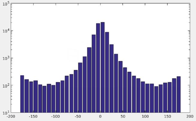
10     Nam N. Vo and James Hays

Fig. 6. Network architecture with data augmentation by random rotation and an ad-
ditional branch that performs orientation regression

generated by data augmentation. As the inference is done on 2 images jointly,
its effect on each individual’s representation can be difficult to interpret. The
motivation, beyond being able to predict query orientation, is that this will make
the network more orientation-aware and therefore produce a better feature rep-
resentation for the localization task.

5    Experiments

Data preparation: we use our dataset of more than 1 million matched pairs of
street-view and overhead-view images randomly collected from Google Maps of
11 different US cities (section 2). We use all the cross-view pairs in 8 cities as
training data (a total of 900k examples) and the remaining 3 cities as 3 test sets
(around 70k examples per set).
    We learn with mini-batch stochastic gradient descent, the standard optimiza-
tion technique for training deep networks. Our batch size is 128 (64 of which are
positive examples while 64 are negative examples). Training starts with a large
learning rate (experimentally chosen) and get smaller as the network converges.
The number of training iterations is 150k. We use Caffe framework [15].
    Data augmentation: we apply random rotation of overhead images during
training and use multiple rotation samples during testing (described in Section
4). The effect will be studied in detail in section 5.2. We also apply a small
amount of random cropping and random scaling.
    Image Ranking and Geolocalization. While we have thus far considered
location matching as a binary classification problem, our end goal is to use it for
geolocalization. This application can be framed as a ranking or retrieval problem:
given a query street view image and a repository of overhead images, one of which
is the match, we want to rank the overhead images according to their relevance
to the query so that the true match image is ranked as high as possible. The
ranking task is typically approached as following: the representation learning
networks are applied to the query image and the repository’s images to obtain
Localizing and Orienting Street Views Using Overhead Imagery 11
Fig. 7. Ranking result examples on the Denver test set (reference set of 70k reference
images)
their feature vectors. Then these overhead images can be ranked by sorting
the distance from their features to the query image’s feature. The localization is
considered successful if the true match overhead image is ranked within a certain
top percentile.
Metrics: we measure both the classification and ranking performance on
each test set. The classification accuracy is computed by using the best threshold
on the each test set (random chance performance is 50%). We found that this
measurement is useful for evaluating classification networks which are hard to
apply to ranking on large test sets because of the computational expense of all-
pairs comparisons through deep networks. For the ranking task, we use mean
recall at top K% as our measurement (the percentage of cases in which the
correct overhead match of the query street view image is ranked within top K
percentile, chance performance is K%). Some ranking examples are shown in
Figure 7.
5.1 Comparison of CNN architectures
We train and compare 6 variants of CNN described in Section 3. All are initialized
from scratch (no pretraining), trained to be 90◦ RI, and tested with 16 rotation
samples. Quantitative comparisons are shown in the top of Table 1.
Not surprisingly, both classification networks achieved better accuracy than
the representation learning Siamese and triplet networks. This is because they
jointly extract and exchange information from both input images. Somewhat12 Nam N. Vo and James Hays
Fig. 8. Histograms of pairwise distances of features produced by the Siamese network-
contrastive loss (left) and the triplet network (right). Note the crowding near zero
distance for the Siamese network, which may explain poor performance for fine-grained
retrieval tasks when it is important to compare small distances.
unexpectedly, in our experiments the hybrid network is the better of the two.
Even-though the ‘pure’ classification network should be capable of producing
the same mapping as the hybrid, it might have trouble learning to process both
images from the 1st layer.
Between the Siamese and triplet network, the triplet network outperforms
the Siamese by a surprisingly large margin on both tasks. While both networks
try to separate matches from non-matches, the contrastive loss function works
toward a secondary objective: drive the distance between matched pair as close
to 0 as possible (Figure 8). Note that this might be a good property for the
learned representation to have; but for the task of matching and ranking we
found that this might compromise the main objective. One way to alleviate this
problem is to add another margin to the contrastive loss function to cut the loss
when the distance is small enough [18].
Table 1. Performance of different networks on different test sets
Task Classification (accuracy) Ranking (recall @top 1%)
Test set Denver Detroit Seattle Denver Detroit Seattle
Section 5.1 experiment (90◦ RI+16rots)
Classification network 90.0 87.8 87.7 N/A N/A N/A
Classification hybrid 91.5 88.7 89.4 N/A N/A N/A
Siamese network 85.6 83.2 82.9 21.6 21.9 17.7
Triplet network 88.8 86.8 86.4 43.2 39.5 35.3
Siamese DBL-Net 90.0 88.0 88.0 48.4 45.0 41.8
Triplet DBL-Net 90.2 88.4 87.6 49.3 47.1 40.0
Section 5.2 (360◦ RI+OR)
DBL-Net + 16rots 91.5 90.1 88.7 54.8 52.7 45.5
DBL-Net + avg16 91.5 90.0 88.8 54.0 52.2 45.3
Section 5.3
Triplet eDBL-Net 91.7 89.9 89.3 59.9 57.8 51.4Localizing and Orienting Street Views Using Overhead Imagery 13
Analysis of Siamese and triplet network’s performance has helped us develop
the DBL layer. As the result, both DBL-Nets significantly outperform the origi-
nal networks. While the Siamese with DBL and triplet network with DBL have
comparable performances, it seems that the triplet DBL-Net is slightly better
at ranking. Note that for most of the experiments we have been conducting, the
performance of these two tasks strongly correlate. We use the triplet network
with DBL layer for all following experiments.
5.2 Rotation invariance
We experiment with partial rotation invariance (RI) and orientation regression
(OR) (described in Section 4) for matching and ranking using the triplet DBL-
Net. The result is shown in Table 2.
Table 2. Comparisons of different amount of partial rotation invariance (RI), with
and without orientation regression (OR), and different numbers of rotation samples
during test time. In this experiment, the triplet network with DBL layer is tested on
the Denver test set. 1GT*: in this setting, we test with 1 overhead image aligned using
the ground-truth orientation (so the network doesn’t have to be RI).
Task Classification (accuracy) Ranking (recall @top 1%)
Number of test rotations 1 4 16 1GT* 1 4 16 1GT*
0◦ RI (no RI) 63.6 68.5 87.2 95.0 11.0 18.8 37.3 76.2
45◦ RI 70.9 86.2 89.9 N/A 19.3 36.8 48.1 N/A
90◦ RI 75.8 89.5 90.2 N/A 24.7 44.7 49.3 N/A
180◦ RI 82.7 89.2 89.6 N/A 31.2 43.0 45.6 N/A
360◦ RI (full RI) 87.7 88.5 88.9 N/A 36.8 40.0 41.9 N/A
90◦ RI + OR 74.3 88.6 89.4 N/A 23.1 43.4 47.4 N/A
360◦ RI + OR 90.9 91.3 91.5 N/A 50.9 53.2 54.8 N/A
360◦ RI + OR + avg16 91.5 N/A N/A N/A 54.0 N/A N/A N/A
As an upper bound, we train a network where overhead images are aligned
to the ground truth camera direction of the street view image (1GT). This
is not a realistic usage scenario for image geolocalization since camera azimuth
would typically be unknown. As expected, the network without RI performs very
well when true alignment is provided during testing (1GT), but performs poorly
otherwise. This baseline shows how challenging the problem has become because
of orientation ambiguity. As the degree of RI during training is increased, the
performance improves.
Observe that fewer numbers of test time rotated crops/samples doesn’t work
well if the amount of RI is limited. The full RI setting is the best when testing
with a single sample. As the number of rotations increase, the performance im-
proves, especially for the partially RI networks. Using 16 rotations, the 90◦ RI
network has the highest performance. It might be the best setting for compro-
mising between invariance and discriminate power (this might not be the case14 Nam N. Vo and James Hays
when using hundreds of samples, but we found that it’s not computationally
practical and the improvement is not significant).
Orientation regression’s impact on the 360◦ RI network is surprisingly signif-
icant; its performance improves by 30% (relatively). However OR doesn’t affect
90◦ RI network positively, suggesting that the 2 techniques might not comple-
ment each other. It’s interesting that the OR is useful even though its effect
during learning is not as intuitive to understand as partial RI. As a by-product,
the network can align matches. The orientation prediction has an average error
of 17◦ for the ground truth matching overhead image and is discussed more in
the supplemental document.
Finally we show the effect of applying multi-orientation feature averaging
on 360◦ RI + OR network. By averaging the feature of 16 samples, we obtain
comparable performance to exhaustively testing with 16 samples (result on all 3
test sets is shown in the 2nd part of Table 1). Though not shown here, applying
this strategy to partial RI networks also slightly improve their performances.
5.3 Triplet sampling by exhausting mini-batch
To speed up the training of triplet networks with the triplet hinge loss, clever
triplet sampling and hard negative mining is usually applied [32, 26, 31]. This is
because the triplet not violating the margin does not contribute to the learning.
However it can skew the input distribution if not handled carefully (for instance,
only mine hardest examples); different schemes were used in [32, 26, 31].
On the other hand, our DBL-log loss is practically a smoothed version of
the hinge loss. We propose to use every possible triplet in the mini-batch. We
experiment with using a mini-batch of 128 pairs of (matched) images. Since
each image in our data has a single unique match only, we can generate a total
of 256 * 127 triplets (256 different anchors, 1 match and 127 non-matches per
anchor). This is done within our exhausting DBL log loss layer implementation
(eDBL); hence the cost of processing the mini-batch is not much more expensive.
In a similar spirit, recent work[23] proposes a loss function that considers the
relationship between every examples in each training batch.
We train a triplet eDBL-Net+360◦ RI+OR+avg16. Its effect is very positive:
the convergence is much faster, after around 30k iterations the network achieved
similar performance as in previous experiments where each network was trained
with 150k iterations using the same batch size. After 80k iterations, we achieve
even better ranking performance, shown at the bottom of table 1.
6 Conclusion
We introduce a new large scale cross-view data of street scenes from ground level
and overhead. On this dataset, we have experimented with different CNN archi-
tectures extensively; the reported results and analysis can be generalized to other
ranking and embedding problems. The result indicates that the Siamese network
with contrastive loss is the least competitive even though it has been popular forLocalizing and Orienting Street Views Using Overhead Imagery 15
cross-view matching. Our proposed DBL layer has significantly improved repre-
sentation learning networks. Last but not least, we show how to further improve
ranking performance by incorporating supervised alignment information to learn
a rotational invariant representation.
Acknowledgments. Supported by the Intelligence Advanced Research
Projects Activity (IARPA) via Air Force Research Laboratory, contract FA8650-
12-C-7212. The U.S. Government is authorized to reproduce and distribute
reprints for Governmental purposes notwithstanding any copyright annotation
thereon. Disclaimer: The views and conclusions contained herein are those of
the authors and should not be interpreted as necessarily representing the official
policies or endorsements, either expressed or implied, of IARPA, AFRL, or the
U.S. Government.
References
1. Agrawal, P., Carreira, J., Malik, J.: Learning to see by moving. In: Proceedings of
the IEEE International Conference on Computer Vision. pp. 37–45 (2015)
2. Altwaijry, H., Trulls, E., Hays, J., Fua, P., Belongie, S.: Learning to match aerial
images with deep attentive architectures. In: Proceedings of the IEEE Conference
on Computer Vision and Pattern Recognition (2016)
3. Bansal, M., Daniilidis, K., Sawhney, H.: Ultra-wide baseline facade matching for
geo-localization. In: Computer Vision–ECCV 2012. Workshops and Demonstra-
tions. pp. 175–186. Springer (2012)
4. Bell, S., Bala, K.: Learning visual similarity for product design with convolutional
neural networks. ACM Transactions on Graphics (TOG) 34(4), 98 (2015)
5. Bromley, J., Bentz, J.W., Bottou, L., Guyon, I., LeCun, Y., Moore, C., Säckinger,
E., Shah, R.: Signature verification using a siamese time delay neural network.
International Journal of Pattern Recognition and Artificial Intelligence 7(04), 669–
688 (1993)
6. Chechik, G., Sharma, V., Shalit, U., Bengio, S.: Large scale online learning of
image similarity through ranking. The Journal of Machine Learning Research 11,
1109–1135 (2010)
7. Chopra, S., Hadsell, R., LeCun, Y.: Learning a similarity metric discriminatively,
with application to face verification. In: Computer Vision and Pattern Recognition,
2005. CVPR 2005. IEEE Computer Society Conference on. vol. 1, pp. 539–546.
IEEE (2005)
8. Dieleman, S., Willett, K.W., Dambre, J.: Rotation-invariant convolutional neural
networks for galaxy morphology prediction. Monthly Notices of the Royal Astro-
nomical Society 450(2), 1441–1459 (2015)
9. Gens, R., Domingos, P.M.: Deep symmetry networks. In: Advances in neural in-
formation processing systems. pp. 2537–2545 (2014)
10. Hadsell, R., Chopra, S., LeCun, Y.: Dimensionality reduction by learning an invari-
ant mapping. In: Computer vision and pattern recognition, 2006 IEEE computer
society conference on. vol. 2, pp. 1735–1742. IEEE (2006)
11. Han, X., Leung, T., Jia, Y., Sukthankar, R., Berg, A.C.: Matchnet: unifying fea-
ture and metric learning for patch-based matching. In: Proceedings of the IEEE
Conference on Computer Vision and Pattern Recognition. pp. 3279–3286 (2015)16 Nam N. Vo and James Hays
12. Hays, J., Efros, A., et al.: Im2gps: estimating geographic information from a single
image. In: Computer Vision and Pattern Recognition, 2008. CVPR 2008. IEEE
Conference on. pp. 1–8. IEEE (2008)
13. He, K., Zhang, X., Ren, S., Sun, J.: Deep residual learning for image recognition.
In: The IEEE Conference on Computer Vision and Pattern Recognition (CVPR)
(June 2016)
14. Huang, J., Feris, R.S., Chen, Q., Yan, S.: Cross-domain image retrieval with a
dual attribute-aware ranking network. In: Proceedings of the IEEE International
Conference on Computer Vision. pp. 1062–1070 (2015)
15. Jia, Y., Shelhamer, E., Donahue, J., Karayev, S., Long, J., Girshick, R., Guadar-
rama, S., Darrell, T.: Caffe: Convolutional architecture for fast feature embedding.
arXiv preprint arXiv:1408.5093 (2014)
16. Ke, Q., Li, Y.: Is rotation a nuisance in shape recognition? In: Proceedings of the
IEEE Conference on Computer Vision and Pattern Recognition. pp. 4146–4153
(2014)
17. Krizhevsky, A., Sutskever, I., Hinton, G.E.: Imagenet classification with deep con-
volutional neural networks. In: Advances in neural information processing systems.
pp. 1097–1105 (2012)
18. Lin, J., Morere, O., Chandrasekhar, V., Veillard, A., Goh, H.: Deephash: Getting
regularization, depth and fine-tuning right. arXiv preprint arXiv:1501.04711 (2015)
19. Lin, T.Y., Belongie, S., Hays, J.: Cross-view image geolocalization. In: Computer
Vision and Pattern Recognition (CVPR), 2013 IEEE Conference on. pp. 891–898.
IEEE (2013)
20. Lin, T.Y., Cui, Y., Belongie, S., Hays, J.: Learning deep representations for ground-
to-aerial geolocalization. In: Proceedings of the IEEE Conference on Computer
Vision and Pattern Recognition. pp. 5007–5015 (2015)
21. Ngiam, J., Chen, Z., Chia, D., Koh, P.W., Le, Q.V., Ng, A.Y.: Tiled convolutional
neural networks. In: Advances in Neural Information Processing Systems. pp. 1279–
1287 (2010)
22. Norouzi, M., Fleet, D.J., Salakhutdinov, R.R.: Hamming distance metric learning.
In: Advances in neural information processing systems. pp. 1061–1069 (2012)
23. Oh Song, H., Xiang, Y., Jegelka, S., Savarese, S.: Deep metric learning via lifted
structured feature embedding. In: The IEEE Conference on Computer Vision and
Pattern Recognition (CVPR) (June 2016)
24. Parkhi, O.M., Vedaldi, A., Zisserman, A.: Deep face recognition. Proceedings of
the British Machine Vision 1(3), 6 (2015)
25. Sangkloy, P., Burnell, N., Ham, C., Hays, J.: The sketchy database: Learning to
retrieve badly drawn bunnies. ACM Transactions on Graphics (proceedings of SIG-
GRAPH) (2016)
26. Schroff, F., Kalenichenko, D., Philbin, J.: Facenet: A unified embedding for face
recognition and clustering. In: Proceedings of the IEEE Conference on Computer
Vision and Pattern Recognition. pp. 815–823 (2015)
27. Shan, Q., Wu, C., Curless, B., Furukawa, Y., Hernandez, C., Seitz, S.M.: Accurate
geo-registration by ground-to-aerial image matching. In: 3D Vision (3DV), 2014
2nd International Conference on. vol. 1, pp. 525–532. IEEE (2014)
28. Sun, Y., Chen, Y., Wang, X., Tang, X.: Deep learning face representation by joint
identification-verification. In: Advances in Neural Information Processing Systems.
pp. 1988–1996 (2014)
29. Taigman, Y., Yang, M., Ranzato, M., Wolf, L.: Deepface: Closing the gap to human-
level performance in face verification. In: Computer Vision and Pattern Recognition
(CVPR), 2014 IEEE Conference on. pp. 1701–1708. IEEE (2014)Localizing and Orienting Street Views Using Overhead Imagery 17
30. Wang, F., Kang, L., Li, Y.: Sketch-based 3d shape retrieval using convolutional
neural networks. In: Proceedings of the IEEE Conference on Computer Vision and
Pattern Recognition. pp. 1875–1883 (2015)
31. Wang, J., Song, Y., Leung, T., Rosenberg, C., Wang, J., Philbin, J., Chen, B., Wu,
Y.: Learning fine-grained image similarity with deep ranking. In: Computer Vision
and Pattern Recognition (CVPR), 2014 IEEE Conference on. pp. 1386–1393. IEEE
(2014)
32. Wang, X., Gupta, A.: Unsupervised learning of visual representations using videos.
In: Proceedings of the IEEE International Conference on Computer Vision. pp.
2794–2802 (2015)
33. Weyand, T., Kostrikov, I., Philbin, J.: Planet - photo geolocation
with convolutional neural networks. CoRR abs/1602.05314 (2016),
http://arxiv.org/abs/1602.05314
34. Workman, S., Souvenir, R., Jacobs, N.: Wide-area image geolocalization with aerial
reference imagery. In: ICCV 2015 (2015)
35. Wu, P., Hoi, S.C., Xia, H., Zhao, P., Wang, D., Miao, C.: Online multimodal deep
similarity learning with application to image retrieval. In: Proceedings of the 21st
ACM international conference on Multimedia. pp. 153–162. ACM (2013)
36. Zagoruyko, S., Komodakis, N.: Learning to compare image patches via convolu-
tional neural networks. In: Conference on Computer Vision and Pattern Recogni-
tion (CVPR) (2015)
37. Zamir, A.R., Shah, M.: Accurate image localization based on google maps street
view. In: Computer Vision–ECCV 2010, pp. 255–268. Springer (2010)
38. Zeiler, M.D., Fergus, R.: Visualizing and understanding convolutional networks.
In: Computer Vision–ECCV 2014, pp. 818–833. Springer (2014)
39. Zhou, B., Lapedriza, A., Xiao, J., Torralba, A., Oliva, A.: Learning deep features
for scene recognition using places database. In: Advances in Neural Information
Processing Systems. pp. 487–495 (2014)Localizing and Orienting Street Views Using Overhead Imagery 1
Supplemental Material: Localizing and Orienting Street
Views Using Overhead Imagery
1 GTCrossView dataset
Figure 1 shows the cities from which we collected data (initially we wanted
to use both big and small city/town, but the image quality seems to be quite
inconsistent).
Majority of the images in the dataset are of rural-like scene because the urban
area is relatively small even in big cities.
Fig. 1. Location of cities we chose to build our dataset. Black: we use for training, and
Red: we use for testing in our experiments.
2 Network visualization
2.1 conv1
Fig. 2. conv1 filters learned by the classification network2 Nam N. Vo and James Hays
First we visualize the first convolutional layer (named conv1 in AlexNet)
learned by these networks. Figure 2 shows conv1 of the learned classification
AlexNet. Since the input of our (modified) network is a 6-channel image, each
convolutional filter also has 6 channels. We split it into 2 parts: channel 1-
3 weights (which apply to street-view image) and channel 4-6 weights (which
apply to overhead image).
A quick observation is that most the weights are (noisy) zero (gray-color)
in either channel 1-3 or 4-6. This indicates that even though this network can
combine and exchange information between 2 images, most filters in the first
layer only focus on extracting feature from 1 image only. To be sure, we compute
the standard deviation of channel 1-3 weights and channel 4-6 weights of each
filter and plot all of them in figure 2-right. Most filters have 1 std higher than
the others and none has both high std value. Another observation is that there’s
more filters focusing on street-view image than overhead image. In fact, the
number of filters having higher channels 1-3 weights std is 111 (out of 192). One
explanation is that the scenes in street-view images have greater variation than
that of overhead images, hence needing more filters’ focus to learn.
Fig. 3. conv1 filters learned by the representation learning network
In figure 3 we show conv1 filters learned by a representation learning networks
are similar. Notice the difference between filters of the street-view image and
overhead image. These filters are similar to their counterpart in the classification
network.
2.2 Output feature activation
It’s difficult to visualize the features learned in the other layers. In object recog-
nition, they usually detect similar objects or objects’ parts [38]. In cross-view
image matching, they detect buildings with similar structural patterns [20]. Our
features from the classification network learn to detect similar scenes (or pairs
of scenes, in case of classification network). Figure 4 shows some images with ex-
treme big value of an output feature in first 5 columns, and images with extreme
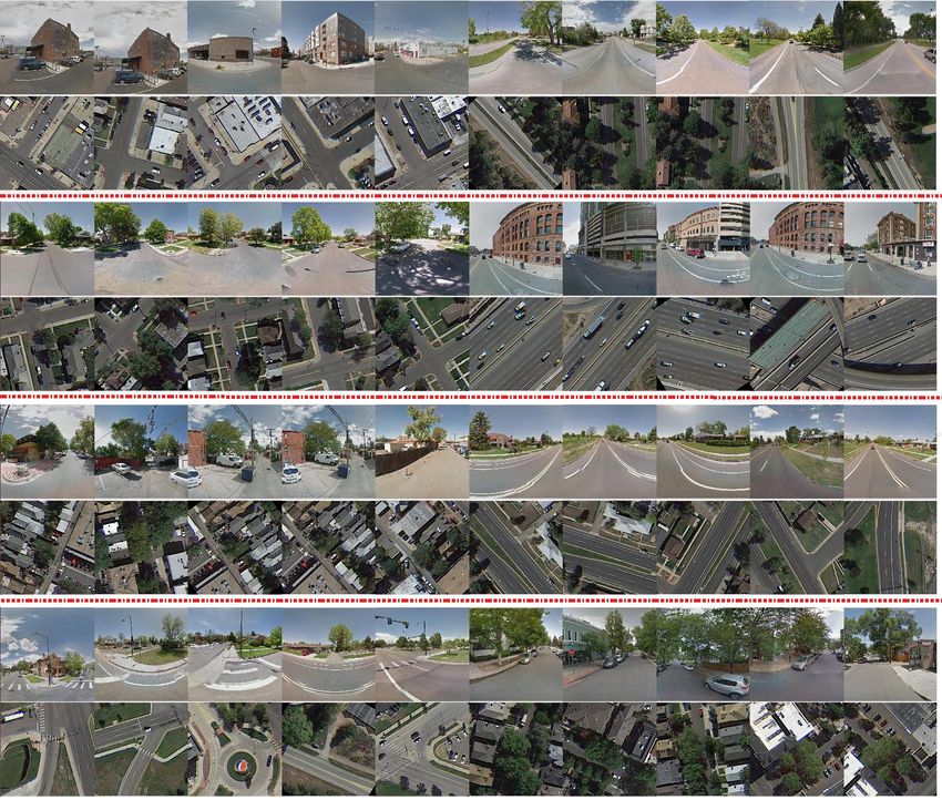
small value of that same feature in the last 5 columns.Localizing and Orienting Street Views Using Overhead Imagery 3 Fig. 4. Examples of images with extreme activation value
4      Nam N. Vo and James Hays

3     Ranking performance
Figure 5 shows the ranking performance of some networks that we have ex-
perimented with (described in the experiment section). The Siamese network
baseline doesn’t perform well relatively suggesting it is not suitable for ranking
application. Each of our proposals (DBL + IR + OR + mini-batch exhausting)
helps to improve the triplet network significantly.

                  Fig. 5. Ranking performance on Denver test set

    In figure 6 we show some image geolocalization examples. Assuming the po-
sition of the overhead images’ scenes is known, we can infer the likely position
of the scene in streetview image.

3.1   Comparison on other datasets (to be updated)
Most state-of-the-arts for verification or ranking using Siamese or triplet network
has been demonstrated to be superior to using shallow or pre-trained features.
Our DBL can help to further improve the performance.
    We experimented on a smaller scale cross-view dataset from [20]. The dataset
has around 80k pairs of matched street view images and aerial images in 7 cities;
the task is to train on 31k pairs and test the ranking performance on the rest.
    We train triplet network and triplet DBL-Net, both initialized from scratch.
With mini-batch exhausting, the network fits really fast and begins to overfit
after only 5k iterations (batch size: 32 pairs). To deal with that we apply heavy
random cropping and random rotation within 10 degree. We run the training
Localizing and Orienting Street Views Using Overhead Imagery 5
Fig. 6. 3 geolocalization examples on the Detroit city test set (85,345 overhead-view
images)
for 30k iterations; the result is shown in table 1. Triplet eDBL-Net seems to
outperform [20] and traditional triplet network on most test sets (though it
might not be directly comparable because our training data is slightly smaller
than what has been originally used in [20]).
Table 1. Ranking performance (Recall at 1%) on [20]’s dataset
Test set SF Charleston Chicago SD Tokyo Rome Lyon
Siamese [20] 22.4 22.6 8.6 23.2 7.3 13.0 11.7
Triplet (e-)Net 26.0 33.1 12.3 24.5 7.3 13.6 8.5
Triplet eDBL-Net 33.8 40.8 18.2 32.0 10.2 17.2 11.1
4 Orientation regression performance
Our network with auxiliary OR loss is capable of predicting the orientation
difference between street-view image and overhead-view image; though it’s only
a by-product and not used for our image geo-localization application. Here we
report the network’s performance on orientation prediction.
We compute the difference (in degree) between the true orientation and the
predicted orientation; the average error (absolute difference) is around 17◦ . We6 Nam N. Vo and James Hays
plot the histogram of these differences on the Denver test set in figure 7. Notice
most fall close to 0◦ , but there’s a very small peak around −180/180◦ . This
represents cases in which the scene looks symmetrical from aerial view point.
We show some examples prediction in figure 8.
Fig. 7. Histograms of difference between predicted orientation and true orientation.
5 Residual network
One can benefit from using deeper network. Here we train a ResNet-101 model
[13] and compare it with AlexNet version, the result is shown in table 2
Table 2. Compare AlexNet vs ResNet-101
Task Classification (accuracy) Ranking (recall @top 1%)
Test set Denver Detroit Seattle Denver Detroit Seattle
eDBL-AlexNet 91.7 89.9 89.3 59.9 57.8 51.4
eDBL-ResNet-101 92.4 91.5 91.5 60.7 64.0 58.4Localizing and Orienting Street Views Using Overhead Imagery 7 Fig. 8. Orientation prediction examples: first row is the street-view images, second row is the ground-truth aligned overhead images and third row is the alignments using predicted orientation.
You can also read