LOCUS 2.0: Robust and Computationally Efficient Lidar Odometry for Real-Time 3D Mapping
←
→
Page content transcription
If your browser does not render page correctly, please read the page content below

IEEE ROBOTICS AND AUTOMATION LETTERS. PREPRINT VERSION. ACCEPTED JUNE, 2022                                                                               1

                                          LOCUS 2.0: Robust and Computationally Efficient Lidar Odometry
                                                           for Real-Time 3D Mapping
                                                            Andrzej Reinke1,2 , Matteo Palieri1,3 , Benjamin Morrell1 , Yun Chang4 , Kamak Ebadi1 ,
                                                                             Luca Carlone4 , Ali-akbar Agha-mohammadi1

                                            Abstract—Lidar odometry has attracted considerable attention
                                         as a robust localization method for autonomous robots operat-
                                         ing in complex GNSS-denied environments. However, achieving
                                         reliable and efficient performance on heterogeneous platforms
                                         in large-scale environments remains an open challenge due to
arXiv:2205.11784v2 [cs.RO] 13 Jun 2022

                                         the limitations of onboard computation and memory resources
                                         needed for autonomous operation. In this work, we present
                                         LOCUS 2.0, a robust and computationally-efficient lidar odom-
                                         etry system for real-time underground 3D mapping. LOCUS
                                         2.0 includes a novel normals-based Generalized Iterative Closest
                                         Point (GICP) formulation that reduces the computation time of
                                         point cloud alignment, an adaptive voxel grid filter that maintains
                                         the desired computation load regardless of the environment’s
                                         geometry, and a sliding-window map approach that bounds
                                         the memory consumption. The proposed approach is shown to
                                         be suitable to be deployed on heterogeneous robotic platforms
                                         involved in large-scale explorations under severe computation
                                         and memory constraints. We demonstrate LOCUS 2.0, a key
                                         element of the CoSTAR team’s entry in the DARPA Subterranean
                                         Challenge, across various underground scenarios.
                                            We release LOCUS 2.0 as an open-source library and also
                                         release a lidar-based odometry dataset in challenging and large-
                                         scale underground environments. The dataset features legged and
                                         wheeled platforms in multiple environments including fog, dust,
                                         darkness, and geometrically degenerate surroundings with a total                 Fig. 1: Four examples from our large underground lidar-based SLAM
                                                                                                                          dataset consisting of over 16 km distance traveled and 11 h of operation
                                         of 11 h of operations and 16 km of distance traveled.                            across diverse environments: (a) a large-scale Limestone Mine (Kentucky
                                           Index Terms—SLAM, Data Sets for SLAM, Robotics in Under-                       Underground), (b) A 3-level urban environment with both large, open spaces
                                         Resourced Settings, Sensor Fusion                                                and tight passages (LA Subway), (c) lava tubes with large vertical changes,
                                                                                                                          and (d) lava tubes with narrow passages. LOCUS 2.0 performed successfully
                                                                                                                          in all these environments on computationally constrained robots.
                                                                   I. I NTRODUCTION                                       preferred over visual sensors to achieve reliable ego-motion
                                                                                                                          estimation in cluttered environments with significant illumina-
                                         L    IDAR odometry has emerged as a key tool for robust
                                              localization of autonomous robots operating in complex
                                         GNSS-denied environments. Lidar sensors do not rely on
                                                                                                                          tion variations (e.g., search, rescue, industrial inspection and
                                                                                                                          underground exploration).
                                         external light sources and provide accurate long-range 3D                           Lidar odometry algorithms aim to recover the robot’s motion
                                         measurements by emitting pulsed light waves to estimate                          between consecutive lidar acquisitions using scan registration.
                                         the range to surrounding obstacles, through time-of-flight-                      Through repeated observations of fixed environmental fea-
                                         based techniques. For these reasons, lidar has been often                        tures, the robot can simultaneously estimate its movement,
                                                                                                                          construct a map of the unknown environment, and use this
                                            Manuscript received: February, 24, 2022; Revised May, 13, 2022; Accepted      map to keep track of its position within it.
                                         May, 19, 2022.
                                            This paper was recommended for publication by Editor Javier Civera upon          While many lidar odometry algorithms can achieve remark-
                                         evaluation of the Associate Editor and Reviewers’ comments.                      able accuracy, their computational cost can still be prohibitive
                                            This work was supported by the Jet Propulsion Laboratory - California         for computationally-constrained platforms, reducing their field
                                         Institute of Technology, under a contract with the National Aeronautics and
                                         Space Administration (80NM0018D0004). This work was partially funded by          of applicability in systems of heterogeneous robots, where
                                         the Defense Advanced Research Projects Agency (DARPA). ©2022 All rights          some of the robots may have very limited computational
                                         reserved.                                                                        resources. Moreover, many existing approaches maintain the
                                            1 Reinke, Palieri, Morrell, Ebadi and Agha-mohammadi are with NASA
                                         Jet Propulsion Laboratory, California Institute of Technology, Pasadena, CA,     global map in memory for localization purposes, making them
                                         USA benjamin.morrell@jpl.nasa.gov                                                unsuitable for large-scale explorations where the map size in
                                            2 Reinke is with University of Bonn, Germany arein@uni-bonn.de
                                            3 Palieri is with the Department of Electrical And Information Engineering,
                                                                                                                          memory would significantly increase.
                                         Polytechnic University of Bari, IT matteo.palieri@poliba.it                         Our previous work [1] presents LOCUS 1.0, a multi-sensor
                                            4 Chang and Carlone are with the Department of Aeronautics and As-            lidar-centric solution for high-precision odometry and 3D
                                         tronautics, Massachusetts Institute of Technology, Cambridge, MA, USA.           mapping in real-time featuring a multi-stage scan match-
                                         lcarlone@mit.edu
                                            Digital Object Identifier (DOI): see top of this page.
                                                                                                                          ing module, equipped with health-aware sensor integration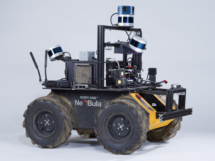
2                                                                  IEEE ROBOTICS AND AUTOMATION LETTERS. PREPRINT VERSION. ACCEPTED JUNE, 2022

that fuses additional sensing modalities in a loosely-coupled                 solution exploiting bundle adjustment over a sliding window of
scheme. While achieving remarkable accuracy and robustness                    lidar scans for enhanced mapping accuracy. While the paper
in perceptually degraded settings, the previous version of                    claims nearly real-time operation, the method does not fuse
LOCUS 1.0: i) had a more significant computational load, ii)                  sensing modalities and maintains the entire map in memory.
maintained the global map in memory, iii) was less robust
to more generalized sensor failures, e.g., failure of one of                  B. Lidar-Inertial Odometry
lidar sensor. LOCUS 2.0 presents algorithmic and system-level
                                                                                 General challenges encountered in pure lidar-based odome-
improvements to decrease the computational load and memory
                                                                              try estimators include degraded motion estimation in high-rate
demand, enabling the system to achieve accurate and real-time
                                                                              motion scenarios [5], and degenerate motion observability in
ego-motion estimation in challenging perceptual conditions
                                                                              geometrically-featureless areas (e.g. long corridors, tunnels)
over large-scale exploration under severe computation and
                                                                              [6], [7]. For these reasons, lidars are commonly fused with
memory constraints.
                                                                              additional sensing modalities to achieve enhanced accuracy in
    The new features and contributions of this work include
                                                                              perceptually-degraded settings [8], [9]. The work [10] presents
(i) GICP from normals: a novel formulation of General-
                                                                              LIO-SAM, an accurate tightly-coupled lidar-inertial odometry
ized Iterative Closest-Point (GICP) that leverages point cloud
                                                                              solution via smoothing and mapping that exploits a factor
normals to approximate the point covariance calculation for
                                                                              graph for joint optimization of IMU and lidar constraints.
enhanced computational efficiency, (ii) Adaptive voxel grid
                                                                              Scan-matching at a local scale instead of a global scale sig-
filter that ensures deterministic and near-constant runtime,
                                                                              nificantly improves the real-time performance. The work [11]
independently of the surrounding environment and lidars, (iii)
                                                                              presents LILI-OM, a tightly-coupled lidar-inertial odometry
improvement and evaluation of two sliding-window map
                                                                              solution with a lidar/IMU hierarchical keyframe-based sliding
storage data structures: multi-threaded octree, ikd-tree [2],
                                                                              window optimization back-end. The work [12] presents LINS,
and (iv) dataset release1 including in challenging, real-world
                                                                              a fast tightly-coupled fusion scheme of lidar and IMU with
subterranean environments (urban, tunnel, cave), shown in
                                                                              error-state Kalman filter to recursively correct the estimated
Fig. 1, collected by heterogeneous robot platforms. All these
                                                                              state by generating new feature correspondences in each
features improve the computational and memory operation
                                                                              iteration. The work [13] presents RTLIO, a tightly-coupled
while maintaining accuracy at the same level. The source code
                                                                              lidar-inertial odometry pipeline that delivers accurate and high-
of LOCUS 2.0 has been released as an open-source library2 .
                                                                              frequency estimation for the feedback control of UAVs by
    The paper is organized as follows. Sec. II reviews related
                                                                              solving a cost function consisting of lidar and IMU residuals.
work on lidar odometry. Sec. III describes the proposed system
                                                                              The work [14] presents FAST-LIO, a computationally-efficient
architecture with a focus on the updates made to the frame-
                                                                              lidar-inertial odometry pipeline that fuses lidar feature points
work to enhance its performance in terms of computational
                                                                              with IMU data in a tightly-coupled scheme with an iterated
load and memory usage. Sec. IV provides an ablation study of
                                                                              extended Kalman filter. A novel formula for computing the
the system on datasets collected by heterogeneous robots dur-
                                                                              Kalman gain results in a considerable decrease of computa-
ing the three circuits of the DARPA Subterranean Challenges,
                                                                              tional complexity with respect to the standard formulation,
an international robotic competition where robots are tasked
                                                                              translating into decreased computation time. The work [15]
to explore complex GNSS-denied underground environments
                                                                              presents DLIO, a lightweight loosely-coupled lidar-inertial
autonomously.
                                                                              odometry solution for efficient operation over constrained
                                                                              platforms. The work provides efficient derivation of local
                        II. R ELATED W ORKS                                   submaps for global refinement constructed by concatenating
   Motivated by the need to enable real-time operation under                  point clouds associated with historical key-frames, along with
computation constraints and large-scale explorations under                    a custom iterative closest point solver for fast and lightweight
memory constraints in perceptually-degraded settings, we re-                  point cloud registration with data structure recycling that
view the current state-of-the-art to assess whether any solution              eliminates redundant calculations. While these methods are
can satisfy these requirements simultaneously.                                computationally efficient, the methods maintain a global map
                                                                              in memory, rendering it unsuitable for large-scale explorations
A. Lidar Odometry                                                             over memory constraints.
   The work [3] proposes DILO, a lidar odometry technique
that projects a three-dimensional point cloud onto a two-                     C. Lidar-Visual-Inertial Odometry
dimensional spherical image plane and exploits image-based                       The work [9] presents Super Odometry, a robust, IMU-
odometry techniques to recover the robot ego-motion in a                      centric multi-sensor fusion framework that achieves accu-
frame-to-frame fashion without requiring map generation. This                 rate operation in perceptually-degraded environments. The
results in dramatic speed improvements, however, the method                   approach divides the sensor data processing into several sub-
does not fuse additional sensing modalities and is not open-                  factor-graphs where each sub-factor-graph receives the predic-
source. The work [4] presents BALM, a lidar odometry                          tion from an IMU pre-integration factor, recovering the motion
    1 https://github.com/NeBula-Autonomy/nebula-odometry-dataset
                                                                              from a coarse to fine manner and enhancing the real-time
    2 https://github.com/NeBula-Autonomy/LOCUS                                performance. The approach also adopts a dynamic octree data
                                                                              structure to organize the 3D points, making the scan-matching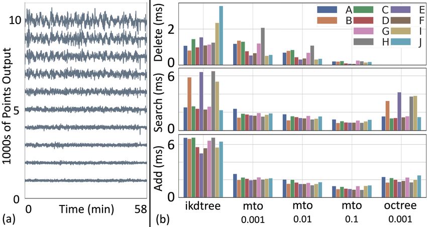
REINKE et al.: LOCUS 2.0                                                                                                                         3

process very efficient and reducing the overall computational                                     Point Cloud Preprocessor
demand. However, the method maintains the global map in              Lidar N     MDC
memory.                                                                                                          Adaptive
                                                                                             Point
                                                                                                        Body      Voxel        Normal
                                                                     Lidar 2     MDC         Cloud
   The work [8] presents LVI-SAM, a real-time tightly-coupled                                Merger
                                                                                                        Filter     Grid      Computation
                                                                                                                  Filter
lidar-visual-inertial odometry solution via smoothing and map-       Lidar 1     MDC
ping built atop a factor graph, comprising a visual-inertial sub-
system (VIS) and a lidar-inertial subsystem (LIS). However,
the method maintains the global map in memory, which it not                                         Scan Matching Unit
                                                                                                                            Point Cloud
                                                                                   Space       Lidar
unsuitable for large-scale explorations with memory limited                                                                   Mapper       Map
                                                                                   Monitor
processing units. The work [16] proposes R2LIVE, an accurate          Odom         Sensor                  Scan-to-          Scan-to-
and computationally-efficient sensor fusion framework for                        Integration                Scan             Submap
                                                                                                                                           Odom
                                                                      IMU          Module      Inital
lidar, camera, and IMU that exhibits extreme robustness to                                     Guess
various failures of individual sensing modalities through filter-
based odometry. While not explicitly mentioned in the paper,                           Fig. 2: LOCUS 2.0 architecture.
the open-source implementation of this method features the           the robot. LOCUS 2.0, in comparison to its predecessor, does
integration of an ikd-tree data structure for map storage which      not recalculate covariances but instead leverages a novel GICP
could be exploited to keep in memory only a robot-centered           formulation to use normals, which only need to be computed
submap.                                                              once and stored in the map (Sec. III-A).
                                                                        In robots with multi-modal sensing, when available, LOCUS
                    III. S YSTEM D ESCRIPTION                        2.0 uses an initial estimate from a non-lidar source (from
                                                                     Sensor Integration Module) to ease the convergence of the
   LOCUS 2.0 provides an accurate Generalized Iterative
                                                                     GICP in the scan-to-scan matching stage, by initializing the
Closest Point (GICP) algorithm [17] based multi-stage scan
                                                                     optimization with a near-optimal seed that improves accuracy
matching unit and a health-aware sensor integration module
                                                                     and reduces computation, enhancing real-time performance, as
for robust fusion of additional sensing modalities in a loosely
                                                                     explained in [1].
coupled scheme. The architecture, shown in Fig. 2, contains
                                                                        LOCUS 2.0 also includes a more efficient technique for map
three main components: i) point cloud preprocessor, ii) scan
                                                                     storage. The system uses a sliding-window approach because
matching unit, iii) sensor integration module. The point cloud
                                                                     large-scale areas are not feasible to be maintained in memory.
preprocessor is responsible for the management of multiple-
                                                                     For example, in one of the cave datasets presented here, a
input lidar streams to produce a unified 3D data product that
                                                                     global map at 1 cm resolution requires 50 GB of memory,
can be efficiently processed by the scan matching unit. The
                                                                     far exceeding the typically available memory on small mobile
preprocessor module consists of Motion Distortion Correction
                                                                     robots. This approach demands efficient computational solu-
(MDC) of the point clouds. This module corrects the distortion
                                                                     tions for insertion, deletion, and search.
in the point cloud from sensor rotation during a scan due to
robot movement using IMU measurements.                               A. GICP from normals
   Next, the Point Cloud Merger enlarges the robot field-of-
view by combining point clouds from different lidar sensors             LOCUS 2.0 uses GICP for scan-to-scan and scan-to-submap
in the robot body frame using their known extrinsic transfor-        matching. GICP generalizes the point-to-point and point-to-
mation. To enable resilient merging of multiple lidar feeds,         plane ICP registration by using a probabilistic model for
we introduce an external timeout-based health monitor that           the registration problem [17]. To do this, GICP requires the
dynamically updates which lidars should be combined in the           availability of covariances for each point in the point clouds
Point Cloud Merger (i.e. a lidar is ignored if its messages          to be aligned. Covariances are usually calculated based on
are too delayed). The health monitoring makes the submodule          the distributions of neighboring points around a given point.
robust to lags and failures of individual lidars so that an output   Segal et al. [17] presents plane-to-plane application with the
product is always provided to the downstream pipeline. Then,         assumption that real-world surfaces are at least locally planar.
the Body Filter removes the 3D points that belong to the             In this formulation, points on surfaces are locally represented
robot. Next, the Adaptive Voxel Grid Filter maintains a fixed        by a covariance matrix, where the point is known to belong
number of voxelized points to manage CPU load and to ensure          to a plane with high-confidence, but its exact location in the
deterministic behavior. It allows the robot to have consistent       plane has higher uncertainty.
computational load regardless of the size of the environment            Here, we show how plane-to-plane covariance calculation
or the number of lidars (or if potential lidar failures). In         is equivalent to calculating covariances from pre-computed
comparison to LOCUS 1.0, the Adaptive Voxel Grid Filter              normals. The fact that only the normal is needed is especially
changes the strategy of point cloud reduction from a blind           important for scan-to-submap alignment since the map would
voxelization strategy with fixed leaf size and random filter         otherwise require recomputing point covariances, which is an
to an adaptive system (Sec. III-B). The Normal Computation           expensive operation involving the creation of a kd-tree and
module calculates normals from the voxelized point cloud.            nearest neighbors search. By instead using normals, the co-
The scan matching unit performs a GICP scan-to-scan and              variance computation is only performed once (since it is not
scan-to-submap registration to estimate the 6-DOF motion of          influenced by the addition of extra points), and the result can
                                                                     be stored and reused.
4                                                        IEEE ROBOTICS AND AUTOMATION LETTERS. PREPRINT VERSION. ACCEPTED JUNE, 2022

   The most common implementations of GICP [18], [19] rely
on computing the covariances CiB and CiA for each point i
in two scans. That calculation of covariances in GICP takes
place as a pre-processing step whenever two scans have to
be registered. In the following, we describe how to obtain
the covariances, without recomputing them every time a scan
is collected. Any well-defined covariance matrix C can be
eigendecomposed to eigenvalues and eigenvectors [20], C =
λ1 u1 · u1 T + λ2 u2 · u2 T + λ3 u3 · u3 T where λ1 , λ2 , λ3 are
the eigenvalues of matrix C, and u1 , u2 , u3 are eigenvectors
of matrix C. Two eigenvalues with the same value can be
interpreted and visualized as eigenvectors that span equally           Fig. 3: Illustration of our our sliding map approach. All points are maintained
2D planar surface with the same distribution in each direction.        until the robot reaches the boundary of the original window (step 3). Then, a
This allows the covariance computation problem to be thought           new window is set, and points outside that window are deleted.
of geometrically.                                                      the variability of the input points that stems from different
   In the plane-to-plane metric, for a point ai from scan A we         sensors configurations and cross-sectional geometry of the
know the position along the normal with very high confidence,          environment. This design goal comes from the fact that almost
but we are less sure about its location in the plane. To represent     all computations in the registration stages are dependent on
this, we set u1 = n, and assign λ1 =  as the variance in the          a number of points N . Therefore the idea is to keep the
normal direction, where  is a small constant. We can then             voxelized number of 3D points fixed to have approximately
choose the other eigenvectors to be arbitrary vectors in the           fixed computation time per scan. The approach is as follows:
plane orthogonal to n and assign them comparatively large              let us take any size of the initial voxel size dinit and set
eigenvalues λ2 = λ3 = 1, indicating that we are unsure about           dleaf = dinit , where dleaf is the size of the voxel leaf in the
location in the plane.                                                 current time stamp. We propose the following control scheme:
   Let us take any vector that lies on the plane and is                dleaft+1 = dleaft NNdesired
                                                                                             scan
                                                                                                   . The formula describes how much
perpendicular to the normal. The vector needs to satisfy               should the current voxel size change dleaft+1 in comparison
the plane equation (that it is perpendicular to the normal             to what the current size is dleaft based on the ratio on the
vector) and cross the origin: nx x + ny y + nz z = 0. Then             number of points in the current input scan Nscan to the points
              n ·x+n ·y
z =        − x nz y , therefore the family of vectors on               that are desired for computation for given robot Ndesired . This
                      (x,y,−(n ·x+n ·y)/n )
the plane is u2 = k(x,y,−(nxx ·x+nyy ·y)/nzz k , where nz and nx       simple technique maintains the number of points on the fixed
corresponds to the component z and x of a normal vector n              level, while avoiding any large jumps in the numbers of points,
and nz = 0 means the horizontal vector. The third vector u3            having too few points (e.g. a faulty scan) or having too many
needs to simultaneously be perpendicular to u1 and u2 since            points. The result is an improvement in the efficiency and
eigenvectors need to span the whole 3D space. Therefore,               reduction of the computational load of the system.
u3 = n × u2 . If we know the eigenvectors and eigenvalues of
matrix C, we have C =  u1 ·u1 T +1.0 u2 ·u2 T +1.0 u3 ·u3 T .         C. Sliding-window Map
Substituting from above, we get:
                                                                          LOCUS 1.0 [1] stored the global map in memory through
             T                T                              T         an octree data structure. The native octree implementation
C = n · n + 1.0 u2 · u2 + 1.0 (n × u2 ) · (n × u2 )
                                                         (1)           does not have an efficient way to prune data out. While a
Then, if we take arbitrarily x = 1 and y = 0 then z = − nnxz ,         possible workaround is to filter the points around the robot and
and the covariance simplifies to:                                      rebuild the octree accordingly, this might be computationally
                                                             T         expensive and lead to long refreshing times.
                     (1, 0, −nx /nz )   (1, 0, −nx /nz )                  To account for these challenges, and enable large-scale
    C = n · nT +                     ·                          (2)
                    k(1, 0, −nx /nz )k k(1, 0, −nx /nz )k              explorations under memory constraints, LOCUS 2.0 provides
                                                         T
              (1, 0, −nx /nz )       (1, 0, −nx /nz )                  two map sliding-window approaches (Fig. 3): i) multi-threaded
      +n ×                      ·n×                                    octree, ii) incremental k-dtree [21] (ikd-tree).
             k(1, 0, −nx /nz )k     k(1, 0, −nx /nz )k
                                                                          Multi-Threaded Octree approach maintains only a robot-
The results mean that the covariance can be purely expressed
                                                                       centered submap of the environment in memory. Two parallel
via precomputed normals at each point.
                                                                       threads (threada and threadb ) each working on dedicated
                                                                       data structures (mapa /octreea and mapb /octreeb ) are respon-
B. Adaptive Voxel Grid Filter                                          sible to dynamically filter the point cloud map around the
    To manage the computation load of lidar odometry, regard-          current robot position through a box-filter, and rebuild the
less of the environment and lidar configuration (in terms of           octree accordingly with the updated map, while accounting
number of lidars and types), we propose an adaptive voxel grid         for robot motions between parallel worker processes.
filter. In this approach, the goal is to maintain the voxelized           Ikd-tree [21] is a binary search tree that dynamically stores
number of points at a fixed level (desired by the user) rather         3D points by merging new scans. Ikd-tree does not maintain
than specifying the voxel leaf size and exposing the system to         3D points only in the leaf nodes: they have points in the
REINKE et al.: LOCUS 2.0 5
TABLE I: Dataset summary.
Distance Duration
ID Place Robot Characteristic lidars
(m) (min)
power plant
feature-poor corridors,
A Elma, WA Husky 631.53 59:56 3
large open spaces
(Urban)
2-level,
power plant
stairs,
B Elma, WA Spot 664.27 32:26 1
feature-poor corridors,
(Urban)
large & narrow spaces
power plant
feature-poor corridors,
(a) NeBula Spot robot (b) NeBula Husky robot
C Elma, WA Husky 757.40 24:21 3*
large & narrow spaces
(Urban)
Fig. 4: Type of robots for heterogeneous robotic system in Nebula framework
Bruceton Mine for DARPA Subterranean Challenge
self-similar
D Pittsburgh, PA Husky 1795.88 65:36 3*
self-repetitive geometries
(Tunnel)
Lava Beds National lava tubes and pools,
3D map (provided by DARPA in the Subterranean Challenge
E Monument, CA Spot 590.85 25:20 non-uniform environment, 1 or produced by the team) is used. The ground-truth trajectory
(Cave) degraded lightning
Bruceton Mine
is produced by running LOCUS 1.0 against the survey-grade
self-similar
F Pittsburgh, PA Husky 1569.73 49:13 3* map (i.e. scan-to-map is scan-to-survey-map). In this mode,
self-repetitive geometries
(Tunnel)
power plant LOCUS 1.0 is tuned for maximum accuracy at the cost of com-
feature-poor corridors,
G Elma, WA Husky 877.21 93:10 3
(Urban)
large & narrow spaces putational efficiency, as it does not need to be run in real-time.
Subway Station
3-level, The ground truth trajectory of the robot is determined based on
multiple stairs,
H Los Angeles, CA Spot 1777.45 46:57
feature-poor corridors,
3 LOCUS 1.0 and its multi-stage registration technique: scan-
(Urban)
large & narrow spaces
to-scan and scan-to-map (with high computational parameters
Kentucky Underground large area,
I Limestone Mine, KY Spot 768.82 19:28 non-uniform environment, 1 and slower pace of data processing) and some manual post-
(Cave) degraded lightning
processing work. These datasets have been made open-source
Kentucky Underground large area,
J Limestone Mine, KY Husky 2339.81 57:55 non-uniform environment, 3 to promote further research on lidar odometry and SLAM
(Cave) degraded lightning
* For our experiments we use only two lidars.
in underground environments: github.com/NeBula-Autonomy/
nebula-odometry-dataset.
internal nodes as well. This structure allows dynamic insertion
and deletion capabilities and relies on lazy labels storage B. Metrics
across the whole data structure. Initial building of an ikd-tree is
For CPU and memory profiling, a cross-platform library for
similar to a kd-tree, where space is split at the median point
retrieving information on running processes and system utiliza-
along the longest dimension recursively. Points that are moved
tion is used [23]. The library is used for system monitoring
out of the boundaries of the ikd-tree data structure are not
and profiling. The CPU represents the percentage value of
deleted immediately, but they are labeled as deleted = T rue
the current system-wide CPU utilization, where 100% means
and maintain information until a rebalancing procedure is
1 core is used. The memory represents statistics by summing
triggered.
different memory values depending on the platform. Odometry
delay measures the difference between odometry message
IV. E XPERIMENTAL R ESULTS creation and the current timestamp of the system. The system
A. Dataset is implemented in Robot Operating System (ROS) framework.
Over the last 3 years, Team CoSTAR [22] has intensively This work considers maximum delay and mean delay since
tested our lidar odometry system in real world environment those two metrics more directly impact the performance of
such as caves, tunnels and abandoned factories. Each dataset the modules using the odometry result, e.g., controllers and
(Tab. I) is selected to contain components that are challenging path planners. Lidar callback time measures the duration time
for lidar odometry. The dataset provides lidar scans, IMU for a scan at the time stamp tk to go through a pipeline of
and wheeled inertial odometry (WIO) measurements, as well processing from the queue of the lidar scans. Scan-to-scan
cameras stream. All datasets have been recorded on differ- time measures the duration time for a scan at time tk to align
ent robotics platforms, e.g., Husky and Spot (Fig. 4) with with a scan at time tk−1 in GICP registration stage. Scan-to-
vibrations and large accelerations as is characteristic of both a submap time measures the duration time for a pre-aligned scan
skid-steer wheeled robot traversing rough terrain and a legged from scan-to-scan at time tk to align with a reference local
robot that slips and acts dynamically in rough terrain. The map in GICP registration.
Husky robot is equipped with 3 on-board VLP16 lidar sensors
extrinsic calibrated (one flat, one pitched forward 30 deg, one C. Computation time
pitched backward 30 deg). The Spot robot is equipped with
1) GICP from normals: The experiments presented in this
one on-board lidar sensor extrinsic calibrated. Spot out-of-
section are designed to show the benefit of GICP from normals
the-box implements (kinematic inertial odometry) KIO and
over GICP and support the claim that this reformulation yields
(visual inertial odometry) V IO, therefore the data records
better computation performance without sacrificing accuracy.
those readouts as well. Lidar scans are recorded at 10 Hz.
For each dataset, we compute statistics over 5 runs. The
WIO and IMU are recorded at 50 Hz. To determine the
GICP parameters for this experiment are chosen based on
ground truth of the robot in the environment, a survey-grade
[24]. The parameters for scan-to-scan and scan-to-submap are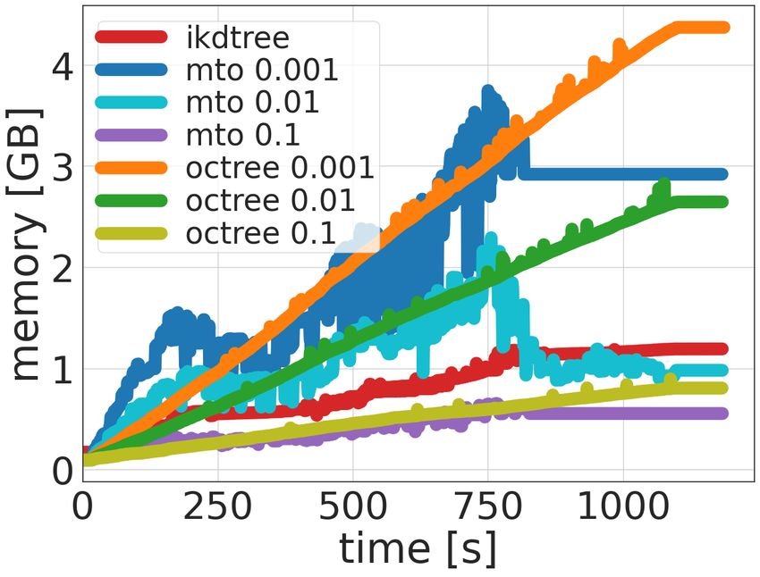
6                                                       IEEE ROBOTICS AND AUTOMATION LETTERS. PREPRINT VERSION. ACCEPTED JUNE, 2022

the same: optimization step 1e−10, maximum corresponding                       TABLE II: Relative memory and CPU change.
distances for associations 0.3, maximum number of iterations
in optimization 20, rotational fitness score threshold 0.005.                   ikd-tree   mto 0.001   mto 0.01   mto 0.1   octree 0.001

Husky computation runs in 4 threads, while Spot uses only 1           Memory   −68.09%     −38.88%     −62.15%    −87.76%        X

thread due to CPU limitations. The octree stores the map with          CPU      9.36%       50.42%     44.36%     19.61%         X

a leaf size 0.001 m.
   The Fig. 5.a-e present the comparison results between GICP       0.001 m is the baseline used in LOCUS 1.0 to maintain full
from normals and GICP across datasets, while Fig. 5.f shows         map information. To assess different parameters mto runs with
the average percentage change across all dataset for each           leaf size 0.1 m, 0.01 m, and 0.001 m.
metric with respect to the GICP method. GICP from normals              For sliding-window approaches, the map size is 50 m
reduces all the computational metrics in LOCUS 2.0: mean            since it is the maximum range of lidars. For scan-to-scan
and max CPU usage, mean and max odometry delay, scan-               and scan-to-submap stage GICP from normals is used with
to-scan, scan-to-submap, lidar callback duration and their          the parameters chosen based on previous experiments. Fig. 9
maximum times. The computation burden is, on average,               presents the maximum memory use for F and I dataset
reduced by 18.57% for all those metrics and datasets. This          and how memory occupation evolves over time. The largest
reduction benefits the odometry update rate since frequency         memory occupancy is for octree and mto version for 0.001 m
increases by 11.10% that is beneficial for another part of          leaf size. The ikd-tree achieves similar performance in terms
the system, i.e. for path planning and control algorithms.          of memory and CPU usage as the mto with leaf size 0.01m.
The lidar callback is generally higher for datasets I and J         Tab. II shows how sliding-window map approaches reduce the
largely due to the consistently large cross-section of Kentucky     memory usage while increasing the CPU usage in comparison
Underground making GICP take longer. One drawback of                to the reference method from LOCUS 1.0.
this method leads to slight increase in the mean and max               Fig. 6.b shows the deletion, insertion and searching proce-
APE errors. The reason is that normals are calculated from          dure timings for different mapping strategies. Ikd-tree has the
sparse point clouds, and those normals are stored in the map        most time-consuming procedures for searching, deletion, and
without any further recomputation. In GICP, the covariances         insertion across all datasets. For insertion, ikd-tree uses on
are recalculated from dense map point clouds. The mean              average 222% more computation time than the octree data
and max APE error increases across all datasets on average          structure as new points need to be stored in a particular
10.82%, but the increase is not for all datasets. Without           manner. For search, ikd-tree gives on average 140% more
including the tunnel dataset (F) the average APE error is only      computation than the octree data structure.
5.23%. The rotational APE errors do not change much since              2) Map size: These experiments show that the size of
max APE decreases 0.94%, while mean APE increases 0.1%.             the sliding map is an important parameter to consider while
                                                                    trading off the computational, memory load and accuracy of
   2) Adaptive Voxel Grid Filter: The second experiment             the result. The sliding-window map allows the system to be
presented in this section shows LOCUS 2.0 adaptive behavior.        bounded by the maximal memory that the robot allocates,
The experiments are run across all datasets with GICP from          following the paradigms of Real-Time Operating System re-
normals and the same parameters as in Sec. IV-C1 with an            quirements. Fig. 10 shows the max APE, CPU and memory
ikd-tree data structure for map maintenance with a box size         metrics for ikd-tree and mto in terms of map size. The smaller
50 m, and Ndesired ranging from 1000 to 10000. Fig. 6.a             map size gives the robot a lower upper bound for the memory,
shows how the adaptive voxel grid filter keeps the number of        but on the other hand, instances with larger maps have lower
points relatively consistent across a 1 hour dataset, no matter     APE as there is more overlap between scan and map. Other
what the input Ndesired is.                                         than memory, these larger maps also see larger the mean and
   There is still some variability in the computation time across   max CPU load.
a dataset, though. Nonetheless, as shown in Fig. 8, the ap-
proach produces a consistent average computation time across        E. Comparison to the state-of-the-art
different environments and sensor configurations, without any          Tab. III shows the comparison study for LOCUS 2.0
large spikes in computation time. This performance gives            against the state-of-the-art methods FAST-LIO [14] and LINS
more predictable computational loads, regardless of robot or        [12] for different environment domains: urban, tunnel, cave
environment, as further reinforced in Fig. 7, where the average     (A,C,F,H,I,J). The table shows that LOCUS 2.0 presents a
callback time and CPU load are similar for all datasets at the      state-of-the-art performance in terms of max and mean APE
same adaptive voxelization setting.                                 error metrics and achieves the smallest errors in 5 out of 6
                                                                    presented datasets. In addition, LOCUS 2.0 is the only method
D. Memory                                                           that does not fail in the tunnel type of the environment (dataset
   1) Map maintenance: The third experiment presented in            F) where lidar slip occurs. In terms of computation, LOCUS
this section presents the benefit of sliding-window maps in         2.0 achieves equivalent performance to FAST-LIO. Memory
real-time systems compared to classic, static octree-based          usage for LOCUS 2.0 is slightly larger, yet this is likely
structures. In these experiments, LOCUS 2.0 uses: ikd-tree          related to the resolution of the map chosen by default in all
and multi-threaded octree (mto). The octree with leaf size          the systems.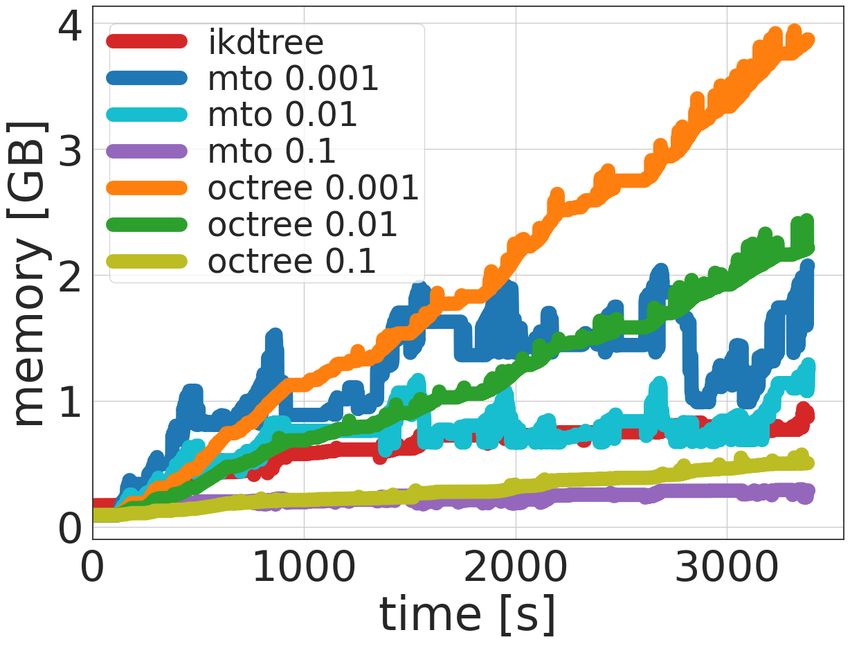
REINKE et al.: LOCUS 2.0                                                                                                                                              7

                Fig. 5: Results of GICP from normals and GICP comparison in LOCUS 2.0. For the meaning of the labels A-J see Tab. I

                                                                                   (a) Husky urban dataset (A).                      (b) Husky cave dataset (J).

Fig. 6: (a) Number of points after the adaptive voxel grid filter for different   Fig. 8: A comparison of the consistency of computation time for adaptive
set-points (on dataset I). (b) Timeplots for deleting, adding, searching for      voxelization with 3000 points and constant leaf size 0.25 (our previously
different map storage mechanisms.                                                 used static voxel size). a) Urban dataset using 2 lidars. b) Cave dataset using
                                                                                  3 lidars.

                                                                                  TABLE III: Comparison of LOCUS 2.0 to the state-of-the art methods
                                                                                  FAST-LIO [14] and LINS [12] for different environment domains.
                                                                                    Dataset   Algorithms             APE                   CPU [%]       max memory
                                                                                                           max [m]     mean [%]          max     mean       [GB]
                                                                                              LOCUS 2.0      0.19            0.09      102.38   185.50      1.06
                                                                                      A       FAST-LIO       0.79           0.30       89.11    126.40       0.36
                                                                                                LINS         0.43           0.18        40.84    81.50      0.42
                                                                                              LOCUS 2.0      0.16            0.24      114.79   198.00      1.30
                                                                                      C       FAST-LIO       2.21           4.22       76.46    307.20      0.99
                                                                                                LINS         0.43           0.60        38.43    75.30       0.47
                                                                                              LOCUS 2.0      0.67            0.45      119.00   229.20      1.98
Fig. 7: The figure presents comparison between adaptive voxelization                  F       FAST-LIO     48555.33        9268.71     156.73   401.30      11.31
                                                                                                LINS        52.73           23.35       28.10    52.30       0.47
1000 − 10000 points and constant leaf size 0.25 (our previously used static
                                                                                              LOCUS 2.0      0.57            0.23      61.05    169.90      2.42
voxel size). For 0.25 voxel the average number points for each dataset (A,            H       FAST-LIO       5.92           5.69       75.15    160.80      0.62
C, D, F, G, J) is 8423, 5658, 2967, 2368, 8511, 15901.                                          LINS        12.11            8.05       39.19    97.90       0.61
                                                                                              LOCUS 2.0      1.39           1.95        72.11   141.60      1.01
                           V. C ONCLUSIONS                                             I      FAST-LIO       0.99           1.44       117.87   167.80       0.80
                                                                                                LINS         0.86            0.85      75.90    101.40      0.85
   This work presents LOCUS 2.0, a robust and computational
                                                                                              LOCUS 2.0      2.42           3.88       107.72   185.00      2.13
efficient lidar odometry system for real-time, large-scale explo-                      J      FAST-LIO       1.72            2.60      126.72   332.50      2.54
                                                                                                LINS         3.56           5.79        73.76   176.50       1.85
rations under severe computation and memory constraints suit-
able to be deployed over heterogeneous robotic platforms. This
work reformulates GICP covariance calculations from precom-                       the computational load independent on the environment and
puted normals that improves the computational performance of                      sensor configuration. Adaptive behavior keeps the number of
GICP. LOCUS 2.0 uses an adaptive voxel grid filter and makes                      points from the lidar consistent while keeping the voxelized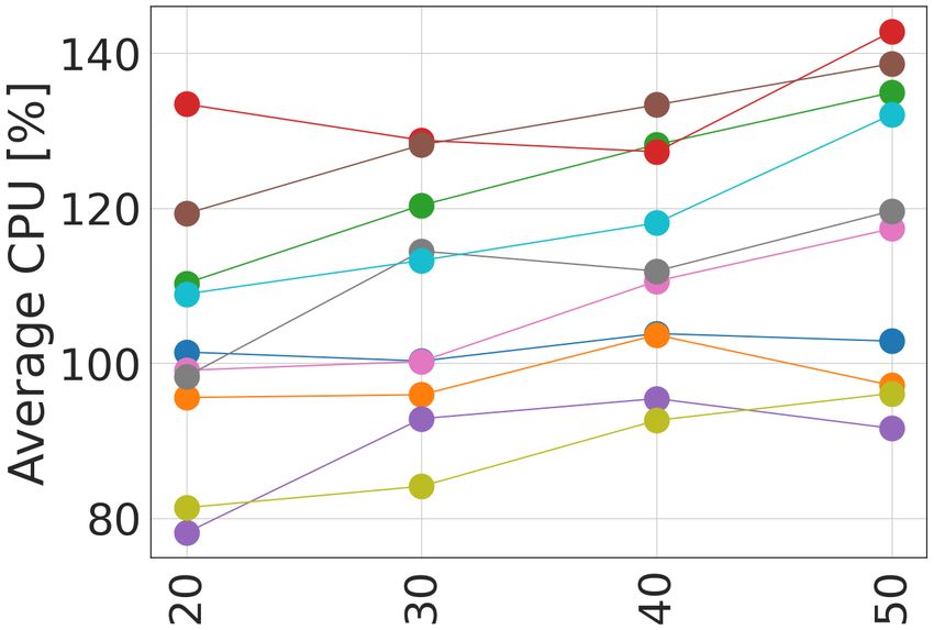
8                                                                     IEEE ROBOTICS AND AUTOMATION LETTERS. PREPRINT VERSION. ACCEPTED JUNE, 2022

                               (a) Husky tunnel (F).

                                 (b) Spot cave (I).

                                                                                    Fig. 10: Results based on size of the map for ikd-tree and mto 0.001 across
                                                                                    all datasets (A-J).
       (c) Memory in time for (F).              (d) Memory in time for (I).          [9] S. Zhao, H. Zhang, P. Wang, L. Nogueira, and S. Scherer, “Super
Fig. 9: The plots show the metrics for different datasets relative to the                odometry: Imu-centric lidar-visual-inertial estimator for challenging
number of fixed voxelized points.                                                        environments,” arXiv preprint arXiv:2104.14938, 2021.
                                                                                    [10] T. Shan, B. Englot, D. Meyers, W. Wang, C. Ratti, and D. Rus, “Lio-sam:
structure of the environment, which stabilizes and improves                              Tightly-coupled lidar inertial odometry via smoothing and mapping,”
the computational load. We evaluate two sliding map strategies                           in 2020 IEEE/RSJ International Conference on Intelligent Robots and
                                                                                         Systems (IROS). IEEE, 2020, pp. 5135–5142.
for reducing memory use: multi-threaded octree and ikd-tree,                        [11] K. Li, M. Li, and U. D. Hanebeck, “Towards high-performance solid-
and show both their computational cost, and improvement in                               state-lidar-inertial odometry and mapping,” IEEE Robotics and Automa-
memory usage. We open-source both LOCUS 2.0, and our                                     tion Letters, vol. 6, no. 3, pp. 5167–5174, 2021.
                                                                                    [12] C. Qin, H. Ye, C. E. Pranata, J. Han, S. Zhang, and M. Liu, “Lins: A
dataset for challenging and large-scale underground environ-                             lidar-inertial state estimator for robust and efficient navigation,” in 2020
ments that features various real-world conditions such as fog,                           IEEE International Conference on Robotics and Automation (ICRA).
dust, darkness, and geometrically degenerate environments                                IEEE, 2020, pp. 8899–8906.
                                                                                    [13] J.-C. Yang, C.-J. Lin, B.-Y. You, Y.-L. Yan, and T.-H. Cheng, “Rtlio:
that restrict mobility. Overall the datasets include 11 h of                             Real-time lidar-inertial odometry and mapping for uavs,” Sensors,
operations and 16 km distance traveled.                                                  vol. 21, no. 12, p. 3955, 2021.
                         R EFERENCES                                                [14] W. Xu, Y. Cai, D. He, J. Lin, and F. Zhang, “Fast-lio2: Fast direct
                                                                                         lidar-inertial odometry,” arXiv preprint arXiv:2107.06829, 2021.
    [1] M. Palieri, B. Morrell, A. Thakur, K. Ebadi, J. Nash, A. Chatterjee,        [15] K. Chen, B. T. Lopez, A.-a. Agha-mohammadi, and A. Mehta, “Direct
        C. Kanellakis, L. Carlone, C. Guaragnella, and A.-a. Agha-Mohammadi,             lidar odometry: Fast localization with dense point clouds,” arXiv preprint
        “Locus: A multi-sensor lidar-centric solution for high-precision odome-          arXiv:2110.00605, 2021.
        try and 3d mapping in real-time,” IEEE Robotics and Automation Letters,     [16] J. Lin, C. Zheng, W. Xu, and F. Zhang, “R2live: A robust, real-time,
        vol. 6, no. 2, pp. 421–428, 2020.                                                lidar-inertial-visual tightly-coupled state estimator and mapping,” arXiv
    [2] Y. Cai, W. Xu, and F. Zhang, “ikd-tree: An incremental kd tree for               preprint arXiv:2102.12400, 2021.
        robotic applications,” arXiv preprint arXiv:2102.10808, 2021.               [17] A. Segal, D. Haehnel, and S. Thrun, “Generalized-icp,” in In Robotics:
    [3] S.-J. Han, J. Kang, K.-W. Min, and J. Choi, “Dilo: Direct light detection        science and systems, vol. 2, no. 4, 2009, p. p. 435.
        and ranging odometry based on spherical range images for autonomous         [18] R. B. Rusu and S. Cousins, “3d is here: Point cloud library (pcl),” in
        driving,” ETRI Journal, vol. 43, no. 4, pp. 603–616, 2021.                       ICRA. IEEE, 2011, pp. 1–4.
    [4] Z. Liu and F. Zhang, “BALM: Bundle adjustment for lidar mapping,”           [19] K. Koide, M. Yokozuka, S. Oishi, and A. Banno, “Voxelized gicp for
        IEEE RAL, vol. 6, no. 2, pp. 3184–3191, 2021.                                    fast and accurate 3d point cloud registration,” EasyChair Preprint no.
    [5] J. Zhang and S. Singh, “Loam: Lidar odometry and mapping in real-                2703, EasyChair, 2020.
        time.” in Robotics: Science and Systems, vol. 2, 2014, p. 9.                [20] G. Strang, Introduction to Linear Algebra, 4th ed. Wellesley, MA:
    [6] A. Tagliabue, J. Tordesillas, X. Cai, A. Santamaria-Navarro, J. P.               Wellesley-Cambridge Press, 2009.
        How, L. Carlone, and A.-a. Agha-mohammadi, “Lion: Lidar-inertial            [21] Y. Cai, W. Xu, and F. Zhang, “ikd-tree: An incremental k-d tree for
        observability-aware navigator for vision-denied environments,” arXiv             robotic applications,” 02 2021.
        preprint arXiv:2102.03443, 2021.                                            [22] A. Agha et al., “Nebula: Quest for robotic autonomy in challenging
    [7] K. Ebadi, M. Palieri, S. Wood, C. Padgett, and A. akbar Agha-                    environments; team costar at the darpa subterranean challenge,” ArXiv,
        mohammadi, “DARE-SLAM: Degeneracy-aware and resilient loop                       vol. abs/2103.11470, 2021.
        closing in perceptually-degraded environments,” Journal of Intelligent      [23] “psutil,” https://psutil.readthedocs.io/en/latest/.
        Robotic Systems, vol. 102, no. 1, pp. 1–25, 2021.                           [24] A. Reinke, “Advanced lidar odometry for exploration of unknown
    [8] T. Shan, B. Englot, C. Ratti, and D. Rus, “Lvi-sam: Tightly-coupled              underground environments,” Master’s thesis, University of Bonn, 2022.
        lidar-visual-inertial odometry via smoothing and mapping,” arXiv
        preprint arXiv:2104.10831, 2021.

You can also read