Machine Source Localization of Tursiops truncatus Whistle-like Sounds in a Reverberant Aquatic Environment - bioRxiv
←
→
Page content transcription
If your browser does not render page correctly, please read the page content below
bioRxiv preprint first posted online Apr. 11, 2019; doi: http://dx.doi.org/10.1101/606673. The copyright holder for this preprint
     (which was not peer-reviewed) is the author/funder, who has granted bioRxiv a license to display the preprint in perpetuity.
                                       It is made available under a CC-BY 4.0 International license.

                                            Machine Source Localization of Tursiops truncatus
                                            Whistle-like Sounds in a Reverberant Aquatic Environment
                                             SF Woodward1 *, D Reiss2 , MO Magnasco1

                                            1 Laboratory of Integrative Neuroscience, Center for Studies in Physics and Biology,
                                            The Rockefeller University, New York, NY, United States
                                            2 Department of Psychology, Hunter College, City University of New York, New York,
                                            NY, United States

                                            * sf.woodward@gmail.com

                                             Abstract
                                             Most research into bottlenose dolphins’ (Tursiops truncatus’ ) capacity for
                                             communication has centered on tonal calls termed whistles, in particular individually
                                             distinctive contact calls referred to as signature whistles. While “non-signature” whistles
                                             exist, and may be important components of bottlenose dolphins’ communicative
                                             repertoire, they have not been studied extensively. This is in part due to the difficulty
                                             of attributing whistles to specific individuals, a challenge that has limited the study of
                                             not only non-signature whistles but the study of general acoustic exchanges among
                                             socializing dolphins. In this paper, we propose the first machine-learning-based
                                             approach to identifying the source locations of tonal, whistle-like sounds in a highly
                                             reverberant space, specifically a half-cylindrical dolphin pool. We deliver time-of-flight
                                             and normalized cross-correlation measurements to a random forest model for
                                             high-feature-volume classification and feature selection, and subsequently deliver the
                                             selected features into linear discriminant analysis, linear and quadratic Support Vector
                                             Machine (SVM), and Gaussian process models. In our 14-point setup, we achieve
                                             perfect classification accuracy and high (0.981 ± 0.802 m) regression accuracy with
                                             fewer than 10,000 features, suggesting an upgrade in accuracy and computational
                                             efficiency to the whole-pool-sampling SRP-PHAT method that is the only competitive
                                             alternative at present, apart from tag-based methods.

                                             Author summary
                                            The common bottlenose dolphin (Tursiops truncatus) has attracted attention as a
                                            distinctly nonhuman, yet intelligent and social species that may be capable of complex
                                            communication. Despite the great interest in probing the “vocal” interactions of
                                            socializing dolphins to evaluate this possibility, a prerequisite to any rigorous attempt is
                                            the matching of vocalizations with their corresponding vocalizers. At present, no
                                            reliable method exists for consistently performing this matching, particularly over long
                                            periods of time and with complete information about the physical condition of all
                                            vocalizers. In this study, we propose the first machine learning-based method for
                                            accomplishing sound localization – the primary step of sound attribution – of
                                            dolphin-like vocalizations in a dolphin pool. On our sample data, this method proves
                                            extremely accurate within the body length of a dolphin, and is suggestive of greater
                                            practical reliability than other available methods.

September 1, 2019                                                                                                                        1/14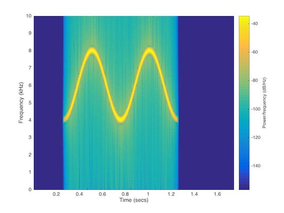
bioRxiv preprint first posted online Apr. 11, 2019; doi: http://dx.doi.org/10.1101/606673. The copyright holder for this preprint
     (which was not peer-reviewed) is the author/funder, who has granted bioRxiv a license to display the preprint in perpetuity.
                                       It is made available under a CC-BY 4.0 International license.

                                             Introduction                                                                                       1

                                            Dolphin communication research is in an active period of growth. Many researchers                   2

                                            expect to find significant communicative capacity in dolphins given their complex social            3

                                            structure [1–3], advanced cognition including the capacity for mirror self-recognition [4],         4

                                            culturally transmitted tool-use and other behaviors [5], varied and adaptive foraging               5

                                            strategies [6], and their capacity for metacognition [7]. Moreover, given dolphins’                 6

                                            well-studied acoustic sensitivity and echolocation ability [8–10], some researchers have            7

                                            speculated that dolphin vocal communication might share properties with human                       8

                                            languages [11–13]. However, there is an insufficiency of work in this area to make                  9

                                            significant comparisons.                                                                            10

                                                Among most dolphin species, a particular tonal class of call, termed the whistle, has           11

                                            been identified as socially important. In particular, for the common bottlenose dolphin,            12

                                            Tursiops truncatus – arguably the focal species of most dolphin cognitive and                       13

                                            communication research – research has focused on signature whistles, individually                   14

                                            distinctive whistles [14–16] that may convey an individual’s identity to                            15

                                            conspecifics [15, 17] and that can be mimicked, potentially to gain conspecifics’                   16

                                            attention [18].                                                                                     17

                                                Signature whistle studies aside, most studies of bottlenose dolphin calls concern               18

                                            group-wide repertoires of whistles and other, pulse-form call types [19–23]; there is only          19

                                            a paucity of studies that seek to examine individual repertoires of non-signature                   20

                                            whistles or the phenomenon of non-signature acoustic exchanges among dolphins.                      21

                                            Regarding the latter, difficulties with sound attribution at best allow for sparse                  22

                                            sampling of exchanges [17, 24]. Nevertheless, such studies constitute a logical                     23

                                            prerequisite to an understanding of the communicative potential of whistles.                        24

                                                The scarcity of such studies can be explained in part by a methodological limitation            25

                                            in the way in which dolphin sounds are recorded. In particular, no established method               26

                                            exists for recording the whistles of an entire social group of dolphins so as to reliably           27

                                            attribute the signals to specific dolphins. The general problem of sound attribution,               28

                                            which is encountered in almost every area of communication research, is typically                   29

                                            approached in one of two ways: (1) by attaching transducers to all potential sound                  30

                                            sources, in which case the source identities of sounds can usually be obtained by                   31

                                            discarding all but the highest-amplitude sounds in each source-distinctive recorder, or             32

                                            (2), by using a fixed array (or arrays) of transducers, a physics-based algorithm for               33

                                            identifying the physical origin of each sound, and cameras that monitor the physical                34

                                            locations of all potential sources for matching.                                                    35

                                                While notable progress has been made implementing attached transducers (or tags)                36

                                            to identify the sources of dolphin whistles [25–27], shortfalls include the need to                 37

                                            manually tag every member of the group under consideration, the tendency of tags to                 38

                                            fall off, and the tags’ inherent lack of convenient means for visualizing caller behavior.          39

                                            On the other hand, a consistently reliable implementation of the array/camera approach              40

                                            to dolphin whistles has not been achieved, even if it has been achieved for dolphin                 41

                                            clicks [28]. In the context of whistles in reverberant environments, authors have noted             42

                                            the complications introduced by multipath effects – resulting from the combination of               43

                                            sounds received from both the sound source and acoustically reflective boundaries – to              44

                                            standard signal processing techniques. These complications generally arise from the                 45

                                            overlap of original and reflected sounds that confound standard, whole-signal methods               46

                                            of obtaining time-of-flight differences. Standard techniques have at best obtained                  47

                                            modest results in relatively irregular, low-reverberation environments where they have              48

                                            been evaluated [29–32]. In unpublished work, we have achieved similar results. One                  49

                                            method of improving a standard signal processing tool for reverberant conditions, the               50

                                            cross-correlation, has been proposed without rigorous demonstration and has not be                  51

                                            reproduced [33]. Among all the methods attempted, one, termed Steer Response Power                  52

September 1, 2019                                                                                                                        2/14
bioRxiv preprint first posted online Apr. 11, 2019; doi: http://dx.doi.org/10.1101/606673. The copyright holder for this preprint
(which was not peer-reviewed) is the author/funder, who has granted bioRxiv a license to display the preprint in perpetuity.
It is made available under a CC-BY 4.0 International license.
Phase Transform (SRP-PHAT), has achieved more success than others (about 40% 53
recall of caller identity), however it relies on a computationally exhausting sampling of 54
all space and has not yet been tested in highly reverberant space [34]. 55
We propose the first machine-learning-based solution to the problem of localizing 56
whistle-like sounds in a highly reverberant environment, a half-cylindrical concrete 57
dolphin pool, located at the National Aquarium in Baltimore, Maryland. We apply it to 58
a broad variety of artificial tonal whistle-like sounds that vary over a range of values 59
within a universally recognized parameter space for classifying dolphin sounds, for a 60
limited number of sampling points. We begin with a random forest classification model 61
and eventually find that a linear classification model that achieves similar results, as 62
well as a regression model that achieves dolphin-length accuracy. The latter two models 63
rely on tight feature sets containing less than 10,000 features to locate a single whistle, 64
and even with preprocessing avoid the computational burden of the full-space 65
cross-correlation sampling required by SRP-PHAT. 66
Materials and methods 67
Sample Set 68
All data were obtained from equipment deployed at the Dolphin Discovery exhibit of 69
the National Aquarium in Baltimore, Maryland. The exhibit’s 110-ft-diameter 70
cylindrical pool is subdivided into one approximate half cylinder, termed the exhibit 71
pool (EP ), as well three smaller holding pools, by thick concrete walls and 6 ft x 4.25 ft 72
(1.83 m x 1.30 m) perforated wooden gates; all pools are acoustically linked. The data 73
were obtained from the EP, when the seven resident dolphins were in the holding pools; 74
their natural sounds were present in recordings. 75
To ensure that the sound samples used for classification were not previously 76
distorted by multipath phenomena (i.e., were not pre-recorded), were obtained in 77
sufficient quantity at several precise, known locations inside the EP, and were 78
representative of the approximate “whistle space” for Tursiops truncatus, we chose to 79
use computer-generated whistle-like sounds that would be played over an underwater 80
Lubbell LL916H speaker. 81
We generated 128 unique sounds (with analysis done on 127) to fill the available 82
time. To be acoustically similar to actual T. truncatus whistles, these sounds were to be 83
“tonal” – describable as smooth functions in time-frequency space, excluding harmonics – 84
and to be defined by parameters and parameter ranges, given in Table 1, representative 85
of those used by field researchers to classify dolphin whistles [35, 36]. To construct a 86
waveform to be played, we began with an instantaneous frequency, f (t), that described 87
a goal time-frequency (or spectrographic) trace, for instance the trace shown in Fig 1. 88
For simplicity, and consistent with the parameters typically used to describe dolphin 89
whistles, we approximated dolphin whistles as sinusoidal traces in spectrographic space – 90
thus f (t) was always a sinusoid. Based on the standard definition of the instantaneous 91
1 dΦ(t)
frequency as f (t) = 2π dt , we obtained the phase Φ(t) by integration of f (t) with 92
respect to time. The phase could be straightforwardly transformed into a playable 93
waveform y(t) as y(t) = A(t)sin(Φ(t)), where A(t) represented a piecewise function that 94
modulated the strength of the signal at different times (the beginning and end of a 95
signal were gradually increased to full intensity and decreased to zero, respectively, as 96
functions of the “Power Onset/Decay Rate,” and the absolute beginning occurred at a 97
peak or trough of the sinusoid f (t) according to “Phase Start”). Alternatively, the phase 98
could be transformed with a heuristic into a waveform that generates a modification of 99
the trace f (t) in spectrographic space, a quasi-sinusoid with “sharpened” peaks and 100
approximate whistle-harmonic-like traces on top of the original trace. This heuristic is 101
September 1, 2019 3/14bioRxiv preprint first posted online Apr. 11, 2019; doi: http://dx.doi.org/10.1101/606673. The copyright holder for this preprint
(which was not peer-reviewed) is the author/funder, who has granted bioRxiv a license to display the preprint in perpetuity.
It is made available under a CC-BY 4.0 International license.
Table 1. Parameters of training set sinusoids.
Parameter Value Set
Duration (sec) [0.3, 1]
Number of Cycles [1, 2 ]
Center Frequency (Hz) [6000, 10500]
Cycle Amplitude (Hz) [2000, 5000]
Phase Start (rad) [− π2 , π2 ]
Power Onset/Decay Rate * [0.1, 0.25]
* Values indicate fraction of signal length over which a sin2 rise/falls occurs.
y(t) = A(t) arcsin(m·sin(Φ(t)))
arcsin(Φ(t)) , where m is a parameter that simultaneously affects the 102
“sharpness” of the peaks and the number of harmonics; we used a value of 0.8. 103
Waveforms were played in Matlab through a MOTU 8M audio interface at calibrated 104
volumes and a rate of 192 kHz. An example of such a sound is given in Fig 1. 105
Fig 1. Spectrogram of an artificial whistle. Displayed is a standard, 1024-bin,
Hamming-window spectrogram of one of the 128 whistle-like sounds that were generated
(and here sampled) at 192 kHz; frequency resolution of the plot is 187.5 Hz. Note that
the spectrogram was constructed from the original, source signal. In this case, Duration
= 1 second, Number of Cycles = 2, Center Frequency = 6000 Hertz, Cycle Amplitude =
2000 Hertz, Phase Start = -π/2.
The 128 sounds were played at each of 14 locations within the EP; they 106
corresponded to 7 unique positions on the water surface on a 3 x 5 cross, at 6 ft (1.83 107
m) and 18 ft (5.49 m) deep. Approximate surface positions are shown in Fig 2; the 108
difference between adjacent horizontal and vertical positions was 10-15 ft (3.05-4.57 m). 109
The LL916H speaker was suspended by rope from a custom flotation device and moved 110
September 1, 2019 4/14bioRxiv preprint first posted online Apr. 11, 2019; doi: http://dx.doi.org/10.1101/606673. The copyright holder for this preprint
(which was not peer-reviewed) is the author/funder, who has granted bioRxiv a license to display the preprint in perpetuity.
It is made available under a CC-BY 4.0 International license.
across the pool surface by four additional ropes extending from the device to research 111
assistants standing on ladders poolside. Importantly, the speaker was permitted to sway 112
from its center point by as much as a meter in arbitrary direction during calibration. 113
These assistants also used handheld Bosch 225 ft (68.58 m) Laser Measure devices to 114
determine the device’s distance from their reference points (several measurements were 115
taken for each location), and through a least-squares trilateration procedure [38] the 116
device location could always be placed on a Cartesian coordinate system common with 117
the hydrophones. Each sound in a 128-sound run was played after a 2-second delay as 118
well as after a 0.25-second, 2-kHz tone, that allowed for the creation of a second set of 119
time-stamps in order to compensate for clock drift during the automated signal 120
extraction. 121
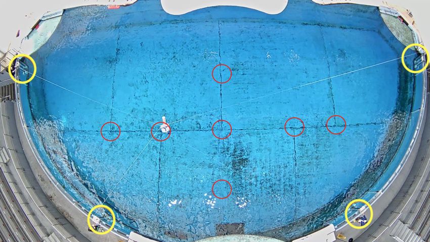
Fig 2. Pool test point and hydrophone array layout. The National Aquarium
Exhibit Pool (EP) is shown, as visualized by the overhead AXIS P1435-LE camera.
Circled in red are the approximate surface projections of the fourteen points (each of
the seven points represents a pair) at which sounds were played. Circled in yellow are
the four hydrophone arrays, each containing four hydrophones.
Recording System 122
Acoustic and visual data was obtained from a custom audiovisual system consisting of 123
16 hydrophones (SQ-26-08’s from Cetacean Research Technology, with approximately 124
flat frequency responses between 200 and 25,000 Hz) split among 4 semi-permanent, 125
tamper-resistant arrays and 5 overhead cameras – for the purpose of this study, only 126
one central AXIS P1435-LE camera, managed by Xeoma surveillance software, was used. 127
The four arrays were spaced approximately equally around the half-circle boundary of 128
the EP (a “splay” configuration). The physical coordinates of all individual 129
hydrophones were obtained by making underwater tape-measure measurements as well 130
as above-water laser-rangefinder measurements; various calibrations were performed 131
that are outside the scope of the present paper. During this test, sounds were collected 132
at 192 kHz by two networked MOTU 8M into the Audacity AUP sound format, to avoid 133
the size limitations of standard audio formats – this system was also used for playing the 134
sounds. Standard passive system operation was managed by Matlab scripts recording to 135
successive WAV files; for consistency Matlab was also used for most data management 136
September 1, 2019 5/14bioRxiv preprint first posted online Apr. 11, 2019; doi: http://dx.doi.org/10.1101/606673. The copyright holder for this preprint
(which was not peer-reviewed) is the author/funder, who has granted bioRxiv a license to display the preprint in perpetuity.
It is made available under a CC-BY 4.0 International license.
and handling. Data is available at https://doi.org/10.6084/m9.figshare.7956212. 137
Classification and Regression 138
1,605 recorded tones were successfully extracted to individual 2-second-long, 16-channel 139
WAV’s that were approximately but not precisely aligned in time. Each tone was 140
labeled with a number designating at which of 14 pool locations it was played. A 141
random 10% of sounds were set aside for final testing, with sinusoids and quasi-sinusoids 142
with the same parameters grouped together given their extreme similarity. 143
Each sound was initially digested into 1,333,877 continuous, numerical features (or 144
variables), together composing the so-called feature set. 145
The first 120 features were time-difference-of-arrivals (TDOA’s) obtained using the 146
Generalized Cross-Correlation Phase Transform (GCC-PHAT) method [39], which in 147
currently unpublished work we found to be most successful among correlation-based 148
methods for obtaining whistle TDOA’s. Briefly, a TDOA is the time difference between 149
the appearance of a signal (such as a whistle) in one sensor (such as a hydrophone) 150
versus another. Possession of a signal’s TDOA’s for all pairs of 4 sensors (with known 151
geometry) in 3-dimensional space is theoretically, but often not practically, sufficient to 152
calculate the exact source position of that signal from geometry [40]. While we establish 153
elsewhere that the 120 TDOA’s (i.e., one TDOA for each distinct pair of our 16 154
hydrophones, excluding self-pairs) obtained from GCC-PHAT are practically not 155
sufficient to calculate the exact source position of our signals using a standard 156
geometric technique that accommodates more than four sensors, Spherical 157
Interpolation [41, 42], we suspected that these TDOA’s might still contain information 158
helpful to a machine learning model. 159
The next 6601 x 136 features consisted of elements from standard, normalized 160
circular cross-correlations [43]: for each unique pair of the 16 hydrophones (including 161
self-pairs), 136 in total, we computed the standard circular cross-correlation of a 162
whistle’s two corresponding audio snippets. While each correlation series was initially 163
384,000 elements long (192,000 samples/second x 2 seconds), we only kept the central 164
6601 elements from each, corresponding to a time-shift range of approximately ±17 165
milliseconds; based on geometry, the first incidence of any sound originating from inside 166
the pool must have arrived within 17 milliseconds between any two sensors (very 167
conservatively), meaning cross-correlation elements corresponding to greater delays 168
could be expected to be less helpful to in-pool source location prediction. 169
Lastly, we included 27,126 x 16 discrete Fourier transform elements (one set for each 170
of 16 hydrophones, for frequencies from 0 Hz to 27,126 Hz). However, preliminary 171
analysis found these features to be universally unhelpful to classification. Thus, they 172
were discarded from the feature set, leaving 897,871 features. 173
Possessing the above feature set for each whistle, each “labeled” by the whistle 174
source location and coordinates, we constructed predictive models on the 90% of 175
whistles made available for model construction (or training). We began with multiclass 176
classification [44], training models to predict which of the 14 possible locations a novel 177
whistle originated from. Given our limited computational resources, our feature set 178
remained too large to accommodate most classifiers. A notable exception was the 179
Breiman random forest [45, 46], which was suitable not only for classification – being a 180
powerful nonlinear multiclass classifier with built-in resistance to overfitting – but for 181
feature reduction (i.e., the process of shrinking feature set size while minimizing loss of 182
classification accuracy), via the permuted variable delta error metric. The permuted 183
variable delta error roughly describes the increase in classification error when a 184
particular feature is effectively randomized, providing a measure of that feature’s 185
importance in classification. We grew a Breiman random forest composed of CART 186
decision trees [47] on the training data; each tree was sequentially trained on a random 187
September 1, 2019 6/14bioRxiv preprint first posted online Apr. 11, 2019; doi: http://dx.doi.org/10.1101/606673. The copyright holder for this preprint
(which was not peer-reviewed) is the author/funder, who has granted bioRxiv a license to display the preprint in perpetuity.
It is made available under a CC-BY 4.0 International license.
√
subset of ˜75% of the training samples using a random ˜ 897, 871 feature subset (as 188
per standard practice). Out-of-bag (OOB) error, referring to the classification error on 189
samples not randomly chosen for the training subset, was used for validation. While an 190
introduction to machine learning is beyond the scope of this paper, these and 191
subsequent techniques are standard with reader-friendly documentation available at 192
such sources as MathWorks (https://www.mathworks.com) and sciikit-learn 193
(https://scikit-learn.org/stable/), to which we direct interested readers. 194
We subsequently used permuted variable delta error as a measure of feature 195
importance, both to examine the selected features for physical significance – recall that 196
cross-correlation element features correspond to pairs of sensors – and to obtain a 197
reduced feature set appropriate for training additional models. On the reduced feature 198
set, we considered a basic CART decision tree [44, 47], a linear and quadratic Support 199
Vector Machine (SVM) [44, 48], and linear discriminant analysis [49]. We also 200
considered Gaussian process regression (also termed kriging) [50, 51] – a nontraditional, 201
nonparametric method of regression that could accommodate our under-constrained 202
data. Whereas the goal of our classification models was to predict which of 14 possible 203
points from which a sound originated, the goal of our regression models was to predict 204
the 3-dimensional coordinates from which the sound originated. 205
We then assessed our ability to locate sounds not originating on the training/testing 206
grid using Gaussian process models. We trained models on training data exclusive of a 207
single grid point, and then evaluated the regression’s performance predicting the 208
coordinates of test sounds from that point. We repeated this process for all grid points 209
and generated statistics. 210
Lastly, we obtained a minimal, nearly sufficient feature set by training a single, 211
sparse-feature (or parsimonious) decision tree classifier on all features of all training 212
data. We then investigated these minimal features for physical significance, by mapping 213
features’ importance (again, using a random forest’s permuted variable delta error) back 214
to the sensor and array pairs from which they derived. 215
Results 216
The random forest trained on the full feature set, as specified above, reached 100.0% 217
OOB accuracy at a size of approximately 180 trees. We continued training to 300 trees, 218
and evaluated the resulting model on the test set: 100.0% accuracy was achieved, with 219
6,788 features possessing permuted variable delta error greater than 0 (based on OOB 220
evaluations). Note that, given the stochastic construction of the random forest, these 221
features did not represent a unique set or superset of sufficient features for obtaining 222
100.0% test accuracy. When we considered which array pairs the 6,778 TDOA and 223
cross-correlation features represented, we found that all pairs of the four hydrophone 224
arrays were represented with no significant preference. 225
We trained several more models on the reduced feature set, including a basic 226
decision tree, a linear and quadratic SVM, and linear discriminant analysis, using 227
10-fold cross-validation. The quadratic SVM as well as linear discriminant analysis 228
achieved 100.0% cross-validation and 100.0% test accuracy, the basic decision tree 229
achieved 96.9% cross-validation and 97.75% test accuracy, and the linear SVM achieved 230
100.0% cross-validation accuracy and 99.44% test accuracy. 231
On the reduced feature set we also performed Gaussian process regression (kriging), 232
generating one model for each spatial dimension. The predicted locations of testing 233
samples for a subset of test locations are plotted in Fig 3. The calculated Euclidean 234
(straight-line) error was 0.981 ± 0.802 m; in the“EP Rear” direction the error was 0.305 235
± 0.375 m, in the ”EP Wall” direction the error was 0.781 ± 0.640 m, and in the “EP 236
Side” direction the error was 0.347 ± 0.574. Comparing the “EP Rear” and “EP Wall” 237
September 1, 2019 7/14bioRxiv preprint first posted online Apr. 11, 2019; doi: http://dx.doi.org/10.1101/606673. The copyright holder for this preprint
(which was not peer-reviewed) is the author/funder, who has granted bioRxiv a license to display the preprint in perpetuity.
It is made available under a CC-BY 4.0 International license.
sets of errors using a two-sided Wilcoxon rank sum test (a non-parametric equivalent of 238
the t-test), the p-value for rejection of the null hypothesis that samples are drawn from 239
distributions with equal medians was 2.02 × 10⁻¹¹ ; between “EP Wall” and “EP Side,” 240
the p-value was 7.89 × 10⁻¹³ ; between “EP Rear” and “EP Side,” the p-value was 241
0.0876. Although standard deviations are indicated above to give the reader some 242
concept of the data spread, we warn the reader that these distributions are not strictly 243
normal according to Anderson-Darling testing. 244
Fig 3. Predictions of test sound locations by Gaussian process regressors.
The half-cylindrical National Aquarium EP is depicted. Large unfilled circles indicate
the true coordinates of the test sounds; each has a unique color. Small filled circles
indicate the test sound coordinates predicted by Gaussian process regression, colors
matching their respective true coordinates.
When the Gaussian process regression models were prompted to predict the 245
coordinates of test sounds from single grid points from which they received no training 246
data, the Euclidean error was significantly greater, at 3.27 ± 0.747 m. In the “EP Rear” 247
direction the error was 0.747 ± 0.689 m, in “EP Wall” direction the error was 2.73 ± 248
0.937 m, and in the “EP Side” direction the error was 0.948 ± 1.01 m. Comparing the 249
“EP Rear” and “EP Wall” sets of errors using a two-sided Wilcoxon rank sum test, the 250
p-value for rejection of the null hypothesis that samples are drawn from distributions 251
with equal medians was 1.10 × 10−48 ; between “EP Wall” and “EP Side,” the p-value 252
was 1.85 × 10−36 ; between “EP Rear” and “EP Side,” the p-value was 0.949. Again, we 253
warn the reader that these distributions are not strictly normal. 254
Next, we trained a single, sparse-feature decision tree on the full training set. The 255
severe feature reduction left 22 features. While the decision tree achieved only 96.63% 256
accuracy on the test set, a random forest trained on the same features achieved 98.88% 257
test accuracy. Thus, we considered this feature set both sufficient and sparse enough to 258
meaningfully ask these features tell us about sensor-sensor pairs a classifier might 259
emphasize. The permuted variable delta error was summed across hydrophone and 260
array pairs, visualized in Fig 4. Overall, we note that, directly or indirectly, features 261
representing all pairs of hydrophone arrays are utilized. 262
Discussion 263
We provided a proof of concept that sound source localization of bottlenose whistles can 264
be achieved implicitly as a classification task and explicitly as a regression task in a 265
September 1, 2019 8/14bioRxiv preprint first posted online Apr. 11, 2019; doi: http://dx.doi.org/10.1101/606673. The copyright holder for this preprint
(which was not peer-reviewed) is the author/funder, who has granted bioRxiv a license to display the preprint in perpetuity.
It is made available under a CC-BY 4.0 International license.
(a) (b)
(c) (d)
Fig 4. Minimal Cross-Hydrophone and Cross-Array Feature Importances.
Aggregate feature importance values for a minimal set of 22 features across hydrophone
and hydrophone array pairs are formed by summing the importances (permuted variable
delta error) of features across hydrophone pairs, and subsequently averaging hydrophone
pair sums across array pairs. a: Cross-hydrophone importances for cross-correlation
features. Hydrophones belonging to common panels (1-4, 5-8, 9-12, 13-16) are grouped
by red boxes. b: Cross-array importances for cross-correlation features. Facing the pool
from the panels increase in number from left to right. c: Cross-hydrophone importances
for TDOA features. d: Cross-array importances for TDOA features.
highly reverberant, half-cylindrical aquatic environment. We began with 127 unique 266
tonal sounds played at 14 positions in the primary dolphin pool at the National 267
Aquarium, recorded with four four-hydrophone arrays. First, we showed that a random 268
forest classifier with less than 200 trees can achieve 100% testing accuracy using 6,788 269
of 897,871 features, including TDOA’s obtained from GCC-PHAT and normalized 270
cross-correlations between all pairs of sensors. We then showed that linear discriminant 271
analysis and a quadratic SVM can achieve the same results on the reduced feature set. 272
If the linear model in particular were to remain valid when trained on a finer grid of 273
training/testing points (finer by about two fold, which would reduce the distance 274
between grid points to approximately the length of a mature bottlenose dolphin), it 275
would constitute a simple and computationally efficient method of locating the origin of 276
tonal sounds in a reverberant environment. 277
Although it remains unclear to what extent sounds originating off-grid are classified 278
to the most logical (i.e., nearest) grid points, a concern even for a classifier trained on a 279
finer grid, we note that our classifiers’ success was achieved despite the few-foot drift of 280
the speaker during play-time; this may indicate a degree of smoothness in the classifiers’ 281
decision-making. Also, that a linear classifier, which by definition cannot support 282
September 1, 2019 9/14bioRxiv preprint first posted online Apr. 11, 2019; doi: http://dx.doi.org/10.1101/606673. The copyright holder for this preprint
(which was not peer-reviewed) is the author/funder, who has granted bioRxiv a license to display the preprint in perpetuity.
It is made available under a CC-BY 4.0 International license.
nonlinear decision making, suffices for this task on features (TDOA’s, cross-correlations) 283
that are generally expected to vary continuously in value across space is reassuring. 284
Nevertheless, this question does warrant further investigation, perhaps with deliberately, 285
faster moving sources. 286
We more suitably addressed the question of off-grid prediction for Gaussian process 287
regression, which was also quite successful when trained on the full training data set, 288
achieving test error of 0.981 ± 0.802 m – less than the expected length of an adult 289
common bottlenose dolphin [52]. Not only is regression inherently suited to 290
interpolation, but it was straightforward to assess regression’s performance on test data 291
from grid points excluded during training. While the regression’s overall performance on 292
novel points was not satisfactory, admitting error larger than average dolphin length at 293
3.27 ± 0.747 m, when we decomposed the error into three dimensions (0.747 ± 0.689 m 294
in ”EP Rear,” 0.948 ± 1.01 m in ”EP Side,” 2.73 ± 0.937 m in ”EP Wall,” with the 295
underlying ”EP Wall” errors significantly different from the other sets of errors by 296
Wilcoxon rank sum testing), we saw that much of the error originated in the direction of 297
pool depth. This is unsurprising given that all data are evenly distributed between only 298
two depths; we would expect a significant boost to performance by introducing 299
additional depth(s) to the data. 300
It also remains unclear to what extent sounds outside the training set, specifically 301
real dolphin whistles, are properly assigned. A test of this would require a large set of 302
dolphin whistles played at known locations in the pool, which we do not possess at 303
present. However, even were an evaluation of real dolphin whistles to fail, we note that 304
in general captive dolphins’ “vocabularies” tend to be limited – groups seem to possess 305
less than 100 unique types [21] – and that it would be realistic to train 306
classification/regression models with whistles closely resembling group members’ sounds, 307
avoiding the need for the model to generalize in whistle type space. 308
We also showed that an extremely sparse, 22-item feature set that lends itself to 309
relatively strong classification accuracy includes time-of-flight comparisons from all four 310
pairs of arrays. As much sound amplitude information was removed in the process of 311
feature creation, this suggests that the decision tree and random forest implicitly use 312
time-of-arrival information for classification from four maximally spaced sensors, 313
consistent with a naive analytic-geometric approach to sound source localization. 314
However, the inner decision making of the models ultimately remains unclear. 315
Overall, we feel this study offers a strong demonstration that machine learning 316
methods are suitable to solving the problem of sound-localization for tonal whistles in 317
highly reverberant aquaria. Were the performance of the methods presented here extend 318
to a finer grid – which was not and will not be feasible in our own work at the National 319
Aquarium, as a result of changes to husbandry policy – they would constitute the most 320
accurate methods to sound source localization of dolphin-whistle-like sounds in a highly 321
reverberant environment yet proposed that avoid the need for tagging; currently, 322
successful localization of whistles in similar environments is no greater than 70% [29–32]. 323
Moreover, as these methods do not require the computation of cross-correlations across 324
the whole sample space, we expect these methods to be less computationally expensive 325
than SRP-PHAT, the primary alternative. With a set of four permanent hydrophone 326
arrays surrounding a subject enclosure, automated overhead tracking, and suitable 327
training set, this method may allow for the creation of a high-fidelity record of dolphin 328
exchanges suitable to statistical analysis in many settings. 329
Acknowledgments 330
We thank the National Aquarium for participating in this study, as well the National 331
Science Foundation (Awards 1530544, 1607280), the Eric and Wendy Schmidt Fund for 332
September 1, 2019 10/14bioRxiv preprint first posted online Apr. 11, 2019; doi: http://dx.doi.org/10.1101/606673. The copyright holder for this preprint
(which was not peer-reviewed) is the author/funder, who has granted bioRxiv a license to display the preprint in perpetuity.
It is made available under a CC-BY 4.0 International license.
Strategic Innovation, and the Rockefeller University for funding. While regrettably we 333
cannot name everyone, we also thank the approximately two dozen people at the 334
National Aquarium, the Rockefeller University, and Hunter College for assisting with 335
various aspects of the project. 336
References
1. Shirihai H, Jarrett B. Whales, Dolphins, and Other Marine Mammals of the
World. Princeton and Oxford: Princeton University Press; 2006.
2. Connor RC, Heithaus MR, Barre LM. Complex social structure, alliance stability
and mating access in a bottlenose dolphin ’super-alliance’. Proceedings of the
Royal Society B: Biological Sciences. 2001;268(1464):263–267.
3. Krutzen M, Sherwin WB, Connor RC, Barre LM, Van de Casteele T, Mann J,
et al. Contrasting relatedness patterns in bottlenose dolphins (Tursiops sp.) with
different alliance strategies. Proceedings of the Royal Society B: Biological
Sciences. 2003;270(1514):497–502.
4. Reiss D, Marino L. Mirror self-recognition in the bottlenose dolphin: A case of
cognitive convergence. Proceedings of the National Academy of Sciences.
2001;98(10):5937–5942.
5. Krutzen M, Mann J, Heithaus MR, Connor RC, Bejder L, Sherwin WB. Cultural
transmission of tool use in bottlenose dolphins. Proceedings of the National
Academy of Sciences. 2005;102(25):8939–8943.
6. Sargeant BL, Mann J, Berggren P, Krutzen M. Specialization and development of
beach hunting, a rare foraging behavior, by wild bottlenose dolphins ( Tursiop
sp.). Canadian Journal of Zoology. 2005;83(11):1400–1410.
7. Smith JD. Inaugurating the Study of Animal Metacognition. International
Journal of Comparative Psychology. 2010;23(3):401–413.
8. Au WWL, Moore PWB, Pawloski D. Echolocation transmitting beam of the
Atlantic bottlenose dolphin. The Journal of the Acoustical Society of America.
1986;80:688–691.
9. Johnson CS. Discussion. In: Busnel RG, editor. Animal Sonar Systems Biology
and Bionics. Jouy-en-Josas, France; 1967. p. 384–398.
10. Au WWL. Echolocation in Dolphins. In: Hearing by Whales and Dolphins. New
York City, New York: Springer; 2000.
11. Lilly JC, Miller AM. Vocal Exchanges between Dolphins. Science.
1961;134(3493):1873–1876.
12. Dreher JJ. Linguistic Considerations of Porpoise Sounds. The Journal of the
Acoustical Society of America. 1961;33(12):1799–1800.
13. McCowan B, Hanser SF, Doyle LR. Quantitative tools for comparing animal
communication systems: information theory applied to bottlenose dolphin whistle
repertoires. Animal Behaviour. 1998;57(2):409–419.
14. Caldwell MC, Caldwell DK. Individualized Whistle Contours in Bottlenosed
Dolphins (Tursiops truncatus). Nature. 1965;207(1):434–435.
September 1, 2019 11/14bioRxiv preprint first posted online Apr. 11, 2019; doi: http://dx.doi.org/10.1101/606673. The copyright holder for this preprint
(which was not peer-reviewed) is the author/funder, who has granted bioRxiv a license to display the preprint in perpetuity.
It is made available under a CC-BY 4.0 International license.
15. Caldwell MC, Caldwell DK, Tyack PL. Review of the
signature-whistle-hypothesis for the Atlantic bottlenose dolphin. In: Leatherwood
S, Reeves RR, editors. The Bottlenose Dolphin. San Diego; 1990. p. 199–234.
16. Sayigh LS, Esch HC, Wells RS, Janik VM. Facts about signature whistles of
bottlenose dolphins, Tursiops truncatus. Animal Behaviour.
2007;74(6):1631–1642.
17. Janik VM, Sayigh LS. Communication in bottlenose dolphins: 50 years of
signature whistle research. Journal of Comparative Physiology A.
2013;199(6):479–489.
18. Tyack PL. Whistle Repertoires of Two Bottlenosed Dolphins, Tursiops truncatus:
Mimicry of Signature Whistles? Behavioral Ecology and Sociobiology.
1986;18(4):251–257.
19. McCowan B. A New Quantitative Technique for Categorizing Whistles Using
Simulated Signals and Whistles from Captive Bottlenose Dolphins (Delphinidae,
Tursiops truncatus). Ethology. 1995;100:177–193.
20. McCowan B, Reiss D. Whistle Contour Development in Captive-Born Infant
Dolphins (Tursiops truncatus): Role of Learning. Journal of Comparative
Psychology. 1995;109(3):242–260.
21. McCowan B, Reiss D. Quantitative Comparison of Whistle Repertoires from
Captive Adult Bottlenose Dolphins (Delphinidae, Tursiops truncatus): a
Re-evaluation of the Signature Whistle Hypothesis. Ethology. 1995;100:194–209.
22. McCowan B, Reiss D, Gubbins C. Social familiarity influences whistle acoustic
structure in adult female bottlenose dolphins (Tursiops truncatus). Aquatic
Mammals. 1998;24(1):27–40.
23. McCowan B, Reiss D. The fallacy of ‘signature whistles’ in bottlenose dolphins: a
comparative perspective of ‘signature information’ in animal vocalizations.
Animal Behaviour. 2001;62(6):1151–1162.
24. Janik VM, King SL, Sayigh LS, Wells RS. Identifying signature whistles from
recordings of groups of unrestrained bottlenose dolphins (Tursiops truncatus).
Marine Mammal Science. 2013;29(1):109–122.
25. Tyack PL. An optical telemetry device to identify which dolphin produces a
sound. The Journal of the Acoustical Society of America. 1985;78(5):1892–1895.
26. Watwood SL, Owen ECG, Tyack PL, Wells RS. Signature whistle use by
temporarily restrained and free-swimming bottlenose dolphins, Tursiops
truncatus. Animal Behaviour. 2005;69(6):1373–1386.
27. Akamatsu T, Wang D, Wang K, Naito Y. A method for individual identification
of echolocation signals in free-ranging finless porpoises carrying data loggers. The
Journal of the Acoustical Society of America. 2000;108(3):1353–5.
28. Watkins WA, Schevill WE. Listening to Hawaiian Spinner Porpoises, Stenella Cf.
Longirostris, with a Three-Dimensional Hydrophone Array. Journal of
Mammalogy. 1974;55(2):319–328.
29. Bell BM, Ewart TE. Separating Multipaths by Global Optimization of a
Multidimensional Matched Filter. IEEE Transactions on Acoustic, Speech, and
Signal Processing. 1986;ASSP-34(5):1029–1036.
September 1, 2019 12/14bioRxiv preprint first posted online Apr. 11, 2019; doi: http://dx.doi.org/10.1101/606673. The copyright holder for this preprint
(which was not peer-reviewed) is the author/funder, who has granted bioRxiv a license to display the preprint in perpetuity.
It is made available under a CC-BY 4.0 International license.
30. Freitag LE, Tyack PL. Passive acoustic localization of the Atlantic bottlenose
dolphin using whistles and echolocation clicks. The Journal of the Acoustical
Society of America. 1993;93(4):2197–2205.
31. Janik VM, Thompson M. A Two-Dimensional Acoustic Localization System for
Marine Mammals. Marine Mammal Science. 2000;16(2):437–447.
32. López-Rivas RM, Bazúa-Durán C. Who is whistling? Localizing and identifying
phonating dolphins in captivity. Applied Acoustics. 2010;71(11):1057–1062.
33. Spiesberger JL. Linking auto- and cross-correlation functions with correlation
equations: Application to estimating the relative travel times and amplitudes of
multipath. The Journal of the Acoustical Society of America.
1998;104(1):300–312.
34. Thomas RE, Fristrup KM, Tyack PL. Linking the sounds of dolphins to their
locations and behavior using video and multichannel acoustic recordings. The
Journal of the Acoustical Society of America. 2002;112(4):1692–1701.
35. Steiner WW. Species-Specific Differences in Pure Tonal Whistle Vocalizations of
Five Western North Atlantic Dolphin Species. Behavioral Ecology and
Sociobiology. 1981;9(4):241–246.
36. Rendell LE, Matthews JN, Gill A, Gordon JCD, MacDonald DW. Quantitative
analysis of tonal calls from five odontocete species, examining interspecific and
intraspecific variation. Journal of Zoology, London. 1999;249:403–410.
37. Weisstein EW. type;. Available from:
http://mathworld.wolfram.com/TriangleWave.html.
38. Navidi W, Jr WSM, undefined, Hereman W. Statistical methods in surveying by
trilateration. Computational Statistics & Data Analysis. 1998;27:209–227.
39. Knapp CH, Carter C. The Generalized Correlation Method for Estimation of
Time Delay. IEEE Transactions on Acoustic, Speech, and Signal Processing.
1976;24(4):320–327.
40. Li X, Deng ZD, Rauchenstein LT, Carlson TJ. Source-localization algorithms and
applications using time of arrival and time difference of arrival measurements.
Review of Scientific Instruments. 2016;87(4):041502–13.
41. Smith JO, Abel JS. The Spherical Interpolation Method of Source Localization.
IEEE Journal of Oceanic Engineering. 1987;OE-12(1):246–252.
42. Zimmer WMX. Passive Acoustic Monitoring of Cetaceans. Cambridge:
Cambridge University Press; 2011.
43. Oppenheim AV, Schafer RW, Buck JR. Discrete-Time Signal Processing. Upper
Saddler River, NJ; 1999.
44. Kotsiantis SB, Zaharakis ID, Pintelas PE. Machine learning: a review of
classification and combining techniques. Artificial Intelligence Review.
2006;26:159–190. doi:10.1007/s10462-007-9052-3.
45. Breiman L. Random Forests. Machine Learning. 2001;45(1):5–32.
46. Belgiu M, Drăguţ L. Random forest in remote sensing: A review of applications
and future directions. ISPRS Journal of Photogrammetry and Remote Sensing.
2016;114:24–31. doi:10.1016/j.isprsjprs.2016.01.011.
September 1, 2019 13/14bioRxiv preprint first posted online Apr. 11, 2019; doi: http://dx.doi.org/10.1101/606673. The copyright holder for this preprint
(which was not peer-reviewed) is the author/funder, who has granted bioRxiv a license to display the preprint in perpetuity.
It is made available under a CC-BY 4.0 International license.
47. Breiman L, Friedman J, Stone CJ, Olshen RA. Classification and Regression
Trees. Monterey, CA: Wadsworth & Brooks/Cole Advanced Books & Software;
1984.
48. Cortes C, Vapnik V. Support-vector networks. Machine Learning.
1995;20:273–297. doi:10.1007/bf00994018.
49. Fisher RA. The use of Multiple Measurements in Taxonomic Problems. Annals of
Eugenics. 1936;7:179–188. doi:10.1111/j.1469-1809.1936.tb02137.x.
50. Wahba G. Spline Models for Observational Data; 1990.
51. Williams CKI. Prediction with Gaussian Processes: From Linear Regression to
Linear Prediction and Beyond. In: Jordan MI, editor. Learning in Graphical
Models. NATO ASI Series (Series D: Behavioural and Social Sciences). vol. 89.
Springer, Dordrecht; 1998.
52. Fernandez S, Hohn AA. Age, growth, and calving season of bottlenose dolphins,
Tursiops truncatus, off coastal Texas. Fishery Bulletin - National Oceanic and
Atmospheric Administration. 1998;(96):357–365.
September 1, 2019 14/14You can also read