Max-Margin Multiple-Instance Dictionary Learning
←
→
Page content transcription
If your browser does not render page correctly, please read the page content below

Max-Margin Multiple-Instance Dictionary Learning

Xinggang Wang†                                                                      wxghust@gmail.com
Baoyuan Wang‡                                                               baoyuanw@microsoft.com
Xiang Bai†                                                                             xbai@hust.edu.cn
Wenyu Liu†                                                                           liuwy@hust.edu.cn
Zhuowen Tu‡,§                                                                   zhuowen.tu@gmail.com
†
  Department of Electronics and Information Engineering, Huazhong University of Science and Technology
‡
  Microsoft Research Asia
§
  Lab of Neuro Imaging and Department of Computer Science, University of California, Los Angeles

                     Abstract                              ing stage, either explicitly or implicitly. For example
    Dictionary learning has became an increas-             the bag of words (BoW) model (Blei et al., 2003), due
    ingly important task in machine learning,              to its simplicity and flexibility, has been adopted in
    as it is fundamental to the representation             a wide variety of applications, in document analysis
    problem. A number of emerging techniques               in particular. In computer vision, the spatial pyramid
    specifically include a codebook learning step,         matching algorithm (SPM) (Lazebnik et al., 2006) has
    in which a critical knowledge abstraction              demonstrated its success in image classification and
    process is carried out. Existing approach-             categorization.
    es in dictionary (codebook) learning are ei-           In this paper, we propose a general dictionary learning
    ther generative (unsupervised e.g. k-means)            method through weakly-supervised learning, in par-
    or discriminative (supervised e.g. extreme-            ticular multiple instance learning (Dietterich et al.,
    ly randomized forests). In this paper, we              1997). Our method can be applied in many domains
    propose a multiple instance learning (MIL)             and here we focus on image-based codebook learning
    strategy (along the line of weakly supervised          for classification. On one hand, visual patterns are giv-
    learning) for dictionary learning. Each code           en as multi-variate variables and often live in high di-
    is represented by a classifier, such as a linear       mensional spaces; on the other hand, there are intrinsic
    SVM, which naturally performs metric fusion            structural information in these patterns, which might
    for multi-channel features. We design a for-           be unfolded into lower dimensional manifolds. Dictio-
    mulation to simultaneously learn mixtures of           nary (codebook) learning provides a way of knowledge
    codes by maximizing classification margins in          abstraction upon which further architectures can be
    MIL. State-of-the-art results are observed in          built.
    image classification benchmarks based on the
    learned codebooks, which observe both com-             In computer vision applications, given a learned code-
    pactness and effectiveness.                            book, each image patch in an input image is either as-
                                                           signed with a code or a distribution (on learned code-
                                                           book); then image representation can be built based
1. Introduction                                            on the encoded image patches. In the experiments of
                                                           this paper, each input sample is denoted by a feature
Finding an effective and efficient representation re-      vector, such as SIFT (Lowe, 2004) and LBP (Ojala
mains as one of the most fundamental problems in ma-       et al., 1996), extracted from an image patch (say 48
chine learning. A number of important developments         × 48). Using codebook has several advantages: (1)
in the recent machine learning literature (Blei et al.,    explicit representations are often enforced; (2) dimen-
2003; LeCun et al., 2004; Hinton et al., 2006; Serre       sionality reduction is performed through quantization;
& Poggio, 2010) have an important dictionary learn-        (3) it facilitates hierarchical representations; (4) spa-
                                                           tial configuration can be also imposed. A direct way to
Proceedings of the 30 th International Conference on Ma-
chine Learning, Atlanta, Georgia, USA, 2013. JMLR:         learning a codebook is by performing clustering, e.g.
W&CP volume 28. Copyright 2013 by the author(s).           the k-means algorithm (Duda et al., 2000). Several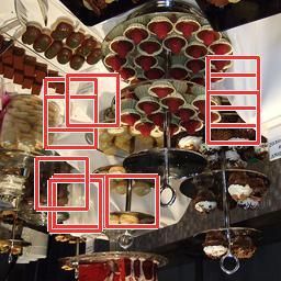
Max-Margin Multiple-Instance Dictionary Learning

                                                               following properties: (1) a multiple instance learning
                                                               strategy is proposed for dictionary learning (an un-
                                                               common direction); (2) each code is represented by a
                                                               linear SVM which naturally performs metric fusion for
                                                               multi-channel features; (3) we design a formulation to
                                                               simultaneously learn mixtures of codes by maximizing
                                                               classification margins in MIL. State-of-the-art results
                                                               are observed in image classification benchmarks with
                                                               significantly smaller dictionary (e.g. only 1/6) than
                                                               the competing methods. Next, we briefly discuss the
                                                               relations between our work and the existing literature
                                                               in dictionary learning.
                     Positive Bag        Negative Bag

                                                               2. Related Work
Figure 1. Illustration of max-margin multiple-instance dic-    Based on low-level descriptors (Lowe, 2004; Ojala
tionary learning. Left: A positive bag containing both
                                                               et al., 1996), bag of words (BoW) model (Fei-Fei &
positive instances (rectangles and diamonds) and negative
instances (circles). In this paper, we assume that positive
                                                               Perona, 2005) using codebooks is widely adapted for
instances may belong to different clusters. We aim to learn    image classification and object detection. On one
max-margin classifiers to separate the instances in positive   hand, unsupervised learning, such as K-means, is al-
bags. Right: A negative bag with all negative instances.       ready demonstrated its popularity for codebook learn-
                                                               ing in many applications. On the other hand, people
                                                               found that supervised learning methods tend to pro-
approaches have been proposed (Jurie & Triggs, 2005;           duce more discriminative codebooks, as described in
Lazebnik & Raginsky, 2009) and one often builds fur-           recent works (Moosmann et al., 2008; Yang et al., 2008;
ther models on top of a learned codebook (Fei-Fei &            2010; Jiang et al., 2012; Mairal et al., 2010; Winn et al.,
Perona, 2005). However, a direct clustering approach           2005). More recently, there are some attempts (Parizi
is often sensitive to: (1) initialization, (2) number of       et al., 2012; Singh et al., 2012; Zhu et al., 2012) tried
codes, and (3) metric (distance) of the multi-channel          to involve latent structures during both the learning
features. In a supervised setting where the labels are         and inference process for image classification, howev-
available, several discriminative codebook learning ap-        er, their target is not for generic dictionary learning.
proaches have also been proposed (Moosmann et al.,             Different from all the previous work, in this paper we
2006; Yang et al., 2008; Moosmann et al., 2008).               try to explicitly perform the dictionary learning along
Instead of learning a dictionary in a fully unsupervised       the line of weakly-supervised learning.
way (e.g. k-means) or supervised way (e.g. random              Strongly supervised methods like Attributes (Farha-
forests (Moosmann et al., 2008)), we take a different          di et al., 2009; Pechyony & Vapnik, 2010; Parikh &
path to dictionary learning through a multiple instance        Grauman, 2011), Poselets (Bourdev & Malik, 2009),
learning strategy. Given a set of training images with         and Object Bank (Li et al., 2010), have shown to
each image assigned with a class label, we treat one           be promising. In our approach, we only use the
particular class of images as positive bags, and the           image-level labels with no additional human annota-
rest images as the negative bags; dense image patches          tions to learn the codebook. In Classemes (Torresani
are collected as the instances in each bag. Our al-            et al., 2010), the emphasis was made on learning an
gorithm then tries to learn multiple linear SVMs for           image-level representation for image search. From the
two purposes: (1) to identify those patches (instances)        viewpoint of multiple instance learning, our proposed
which are genuine to the class of interest; (2) to learn       method is related to multiple component learning (M-
linear SVM classifiers to classify those identified patch-     CL) (Dollár et al., 2008) and multiple clustered in-
es. These linear SVMs naturally cluster the positive           stance learning (MCIL) (Xu et al., 2012). Due to
instances into different clusters. We repeat the pro-          the lack of explicit competition among the clusters,
cess for all the image classes and collect the learned         however, both MCL and MCIL are hard to general-
classifiers, which become our dictionary (codebook).           ize to solve the codebook learning problem. From the
Due to the difference to the codes learned in standard         viewpoint of multiple instance clustering, our proposed
ways, we call each learned linear SVM as generalized           method is related to M3 MIML (Zhang & Zhou, 2008)
code, or G-code. In this paper, we propose a learning          and M3 IC (Zhang et al., 2009) methods. However,
framework to achieve the above goal, which has the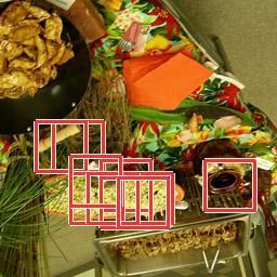
Max-Margin Multiple-Instance Dictionary Learning

both M3 MIML and M3 IC try to maximize the bag-
                                                                  Given positive bags and negative bags, do the follow-
level margin, we instead maximize the instance-level              ing two steps.
margin with the MIL constrains, which is quite dif-
ferent from (Zhang & Zhou, 2008; Zhang et al., 2009)              MIL step: Run mi-SVM on the input positive and
in problem formulation, research motivation, and task                negative bags, and obtain positive instances in
                                                                     positive bags.
objective.
                                                                  Clustering step: Run k-means on the positive in-
                                                                      stances obtained by mi-SVM.
3. Max-margin Multiple-Instance
   Dictionary Learning
                                                                Figure 2. A naive solution for multiple-instance dictionary
3.1. Notation and Motivation
                                                                learning.
We first briefly give the general notations of MIL (Di-
etterich et al., 1997). In MIL, we are given a set of
bags X = {X1 , . . . , Xn }, each of which contains a set       lem.
of instances Xi = {xi1 , . . . , xim }; and each instance
is denoted as a d-dimensional vector xij ∈ Rd×1 . In            3.2. A Naive Solution
addition, every bag is also associated with a bag la-
bel Yi ∈ {0, 1}; and every instance is associated with          A naive way to use MIL for dictionary learning is to
an instance label yij ∈ {0, 1} as well. The relation            first run the standard MIL (e.g. mi-SVM) to select
between bag label and instance labels is interpreted            positive instances, then run a clustering algorithm to
in the following way: if Yi = 0, then yij = 0 for all           build the dictionary. In Fig. 2, we show a naive solu-
j ∈ [1, . . . , m], i.e., no instance in the bag is positive.   tion based on the mi-SVM (Andrews et al., 2002) and
If Yi = 1, then at least one instance xij ∈ Xi is a             k-means algorithm. This method typically treats mul-
positive instance of the underlying concept.                    tiple instance learning and mixture models learning
                                                                as two independent steps, which is not necessarily the
To use MIL for dictionary learning, we consider an im-          optimal solution. In the following, we will introduce
age as a bag, and a patch (or region) within the image          our formulation to perform these two steps simulta-
as an instance. Given a set of images from multiple             neously, which is called max-margin multiple-instance
classes with the corresponding class labels, we treat           dictionary learning (MMDL).
the images of one typical class as positive images, and
the rest ones as negative images. Intuitively, for each         3.3. Formulation of MMDL
image, if it is labelled as positive, then at least one
patch within it should be treated as a positive patch;          In MMDL, we explicitly maximize the margins be-
while if it is labelled as negative, then all patches with-     tween different clusters. To achieve this goal, we build
in it should be labeled as negative patches. Take the           the MMDL based on multi-class SVM, e.g., Crammer
images in 15 Scene dataset (Lazebnik et al., 2006) as           and Singer’s multi-class SVM in (Crammer & Singer,
an example, if highway class is the positive class, then        2002). Without loss of generality, we simply adapt the
the mountain class falls into the negative class; image         linear classifier, which is defined as f (x) = wT x. Each
patches of sky appear in both classes will be treated as        cluster is then associated with a specific linear classi-
negative patches. As shown in Fig. 1, we assume pos-            fier. Due to the flexibility introduced by the multi-
itive patches are drawn from multiple clusters, and we          class SVM formulation, it’s very natural to allow all
view negative patches from a separate negative cluster.         the classifiers to compete with each other during the
The goal of this paper is to learn max-margin classi-           learning process. In this paper, we introduce a cluster
fiers to classify all patches into different clusters, and      label as latent variable, zij ∈ {0, 1, . . . , K}, for each in-
illustrate the learned classifiers (G-codes) for image          stance. If zij = k ∈ {1, . . . , K}, instance xij is in the
categorization/classification. Our dictionary learning          kth positive cluster. Otherwise, zij = 0, xij is in the
problem involves two subproblems: (1) discriminative            negative cluster. Furthermore, we also define a weight-
mixture model learning and (2) automatic instance la-           ing matrix W = [w0 , w1 , . . . , wK ], wk ∈ Rd×1 , k ∈
bel assignment (which cluster a patch might belong              {0, 1, . . . , K} as linear classifiers stacked in each colum-
to). It seems that MIL is a natural way to address              n, where wk represents the k-th cluster model. Note
the above problem. Hence, in the following, we will             that, w0 denotes the negative cluster model. Hence,
first give a naive solution, and then provide detailed          instance xij can be classified by:
formulation and solution to our proposed max-margin
multiple-instance dictionary learning (MMDL) prob-                                 zij = arg maxk wkT xij                  (1)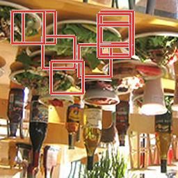
Max-Margin Multiple-Instance Dictionary Learning

 Input: Positive bags, negative bags, and the number of positive clusters K.
 Initialization: For instances in negative bags, we set zij = 0. For instances in positive bags, we use k-means algorithm
 to divide all these instances into K clusters, and set cluster label to be index of clustering center. Instance weight is
 set to 1, pij = 1, for all instances in positive bags.
 We iterate the following two steps for N ( N is typically set to 5 in our experiments) times:
    Optimize W: we sample ps portion of the instances per positive bag according to instance weight pij and take
     all negative instances to form a training set D0 ; since cluster labels are known, we solve the multi-class SVM
     optimization problem to obtain W,
                                               K
                                               X                  X
                                         min         k wk k2 +λ        max(0, 1 + wrTij xij − wzTij xij )
                                          W
                                               k=0                ij

         in which xij ∈ D0 and rij = arg maxk∈{0,...,K},k6=zij wkT xij .

    Update pij and zij : for all instances in positive bags:
      1. Update pij according to Eq. (4)
      2. Update zij = arg maxk∈{1,...,K} wkT xij − w0T xij


 Output: The learned classifiers W.

                                            Figure 3. Optimization algorithm for MMDL

With the above definitions, the objective function be-                   lem is even harder, since we do not know the number
comes                                                                    of positive instances in each positive bag.
           K
           X                    X
 min             k wk k2 +λ          max(0, 1 + wrTij xij − wzTij xij ) 3.4. Learning Strategies of MMDL
W,zij
           k=0                  ij
                       X                                                 At first, we denote training set as D = {X1 , . . . , Xn }
  s.t.    if Yi = 1,       zij > 0, and if Yi = 0, zij = 0,              including all positive and negative bags for training.
                       j                                                 Then we define instance weight as follows:
                                                       (2)
where rij = arg maxk∈{0,...,K},k6=zij wkT xij .
                                                                                                         wkT xij − w0T xij /σ)

                                                                         pij = sigmoid(       max
                             PK                                                            k∈{1,...,K}
                                                2
In Eq. (2), the first term,    k=0 k wk k is for the                                                                               −1
margin regularization, while the second term is the                                                           wkT xij − w0T xij /σ

                                                                             = 1 + exp −            max
multi-class hinge-loss denoted as `(W; (xij , zij )).                                           k∈{1,...,K}

                      X                                                                                                       (4)
 `(W; (xij , zij )) =   max(0, 1 + wrTij xij − wzTij xij )               pij shows “positiveness” of the instance. It is deter-
                           ij                                            mined by the maximal difference of SVM decision func-
                                                    (3)                  tion value between a positive cluster and the negative

Parameter λ controls the relative importance between                     cluster which is maxk∈{1,...,K} wkT xij − w0T xij . Sig-
the two terms. The loss function `(W; (xij , zij )) ex-                  moid function is used for mapping the difference of
plicitly maximizes soft-margins between all K +1 clus-                   SVM decision function value into the range of (0, 1).
ters. Constraints in Eq. P (2) are equivalent
                                           P to con-                     σ is a parameter for normalization.
straints in MIL. Because j zij > 0 ⇔         j yij > 0                   In the next step, we solve the problem in (2) using
and zij = 0 ⇔ yij = 0.
                                                                         coordinate descend in a stochastic way which is sum-
This MMDL formulation leads to a non-convex op-                          marized in Fig. 3. We form a new training set D0 out
timization problem. However, this problem is semi-                       of the original D by sampling instances from each bag
convex (Felzenszwalb et al., 2010) since optimization                    based on pij . Because latent variables are only effec-
problem becomes convex once latent information is                        tive for instances in positive bags, we take all instances
specified for the instances in the positive bags. In                     in negative bags into D0 . In addition, we only sample
(Felzenszwalb et al., 2010), a “coordinate descend”                      ps portion of the instances per positive bag. Initially,
method is proposed to address this kind of problem,                      the instance weights are equal for all positives. After
which guarantees to give a local optimum. Our prob-                      the sampling step, the data set D00 is used to train
Max-Margin Multiple-Instance Dictionary Learning

        street             highway                    coast                                 the kth G-code is wkT x, k ∈ {0, 1, . . . , K}. Thus, we
        class                class                    class                                 can obtain a response map for each G-code classifier.
 Training images                                                                            For each response map, a three-level spatial pyramid
                            MMDL                                                            representation (Lazebnik et al., 2006) is used, resulting
    patches
                                                                                            in (12 + 22 + 42 ) grids; the maximal response for each
                                                                                            G-code classifier in each grid is computed, resulting in
                                                                                            M ×(K +1) length feature vector for each grid. A con-
                                                                                            catenation of features in all grids leads to a compact
 Clusters
                                                                                            image descriptor of the input image.
                   G-code classifier responses
                                                              Max classification response
                                                                                            Note that the complexity of feature encoding using
                                                 response
                                                                                            G-codes is very low. It involves no more than a dot
                                                                  G-code classifier         product operation. The benefit of using G-codes of
 Input image                                                Image representation
                                                                                            low complexity is evident, since feature encoding is a
                         Spatial pyramid
                                                                                            time-consuming process in many classification system-
                                                                                            s (Chatfield et al., 2011). For the high-level image
Figure 4. Illustration of MMDL for image classification.                                    classification tasks, our image representation achieves
Given a set images (in the first row) from multiple classes,                                the state-of-the-art performance on several benchmark
we divide image patches into different clusters and obtain                                  datasets.
G-codes through MMDL. Some patches in the learned clus-
ters (both positive and negative) are shown in the second
row. For an input image, image representation is build                                      5. Experiments
based on response maps of G-code classifiers and spatial
pyramid (shown in the third row).                                                           Dataset We evaluate the proposed MMDL method
                                                                                            for image classification on three widely used dataset-
                                                                                            s, including scene image (15 Scene (Lazebnik et al.,
                                                                                            2006), MIT 67 Indoor (Quattoni & A.Torralba, 2009)
a standard multi-class SVM classifier f0 . This com-                                        datasets), activity images (UIUC Sports dataset (Li
pletes the Optimize W step. Once we get f0 , we                                             & Fei-Fei, 2007)). Experimental setting for the three
can apply it to the original positive bags to perform                                       datasets are listed below:
Update pij and zij step. Then, we sample another
ps portion of instances from each positive bag based                                          • 15 Scene: It contains 4,485 images divided into 15
on the classification results, forming a new dataset D10                                        categories, each category has 200 to 400 images,
and then obtain f1 . This process is repeated until the                                         and the average image size is 300 × 250. Follow-
desired number of iterations N is reached. Sampling                                             ing the same experimental setup as in (Lazebnik
instances according to their “positiveness” makes sure                                          et al., 2006), we take 100 images per class for
that a portion of instances in positive bag have pos-                                           training and use the remaining images for test-
itive instance labels. This satisfies the constraint in                                         ing.
Eq. (2). In addition, this sampling procedure can also
                                                                                              • MIT 67 Indoor: This dataset contains images
increase the efficiency of our optimization algorithm.
                                                                                                from 67 different categories of indoor scenes.
                                                                                                There is a fixed training and test set containing
4. MMDL for Image Representation                                                                approximately 80 and 20 images from each cate-
                                                                                                gory respectively.
A learned dictionary consists of a set of linear clas-
sifiers (G-code classifiers) for different patch clusters                                     • UIUC Sports: This is a dataset of 8 event classes.
from different image classes. Similar to the way in ob-                                         Seventy randomly drawn images from each class
ject bank (Li et al., 2010), our image representation                                           are used for training and 60 for testing follow-
is constructed from the responses of G-code classifiers.                                        ing (Li & Fei-Fei, 2007).
Our MMDL framework is illustrated in Fig. 4. Sup-
pose there are M categories in the dataset, for each                                        For the 15 Scene and UIUC Sports datasets, we ran-
image category, we use the training images in this cat-                                     domly run experiments for 5 times, and record average
egory as positive examples, and the rest training im-                                       and standard deviation of image classification accura-
ages as negative examples. Through MMDL, K + 1                                              cies over all image classes.
G-code classifiers are learned. Given an input image,
patch-level image features are densely extracted. Sup-                                      Experiment Setup For each image, image patches
pose x is a local feature vector, response of x given by                                    are densely sampled by every 16 pixels on image, under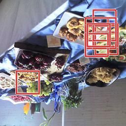
Max-Margin Multiple-Instance Dictionary Learning

three scales, 48×48, 72×72, and 96×96. For each im-                                          88
age patch, we resize it to 48×48 and compute five kind-
s of features for describing it. The features are HoG,                                       86

                                                               Classification accuracy (%)
LBP, GIST (Oliva & Torralba, 2001), encoded SIFT                                             84
and LAB color histogram. For the HoG and LBP fea-
                                                                                             82
tures, we use the implementation in VLFeat (Vedaldi                                                                               HoG + MMDL
& Fulkerson, 2008); their dimensions are 279 and 522,                                        80                                   LBP + MMDL
respectively. For the GIST feature, we use the imple-                                                                             GIST + MMDL
                                                                                             78
mentation provided by the authors of (Oliva & Torral-                                                                             Encoded SIFT + MMDL
                                                                                                                                  Multi-features + MMDL
ba, 2001); its dimension is 256. When computing the                                          76
                                                                                                                                  mi-SVM + k-means
encoded SIFT feature, we densely compute SIFT fea-                                           74                                   k-means
ture at the size of 16 by every 6 pixels; then the SIFTs                                                                          ERC-Forests
are quantized by a 100 bins via k-means by assigning                                         72
                                                                                                  0   200   400   600   800   1000 1200 1400 1600 1800 2000 2200

each SIFT feature to its nearest entry in the cluster;                                                            Number of codewords
a histogram is built on the quantized SIFTs; dimen-
sion of the encoded SIFT feature is 100. For the LAB       Figure 5. Average classification accuracies of different
color histogram feature, we compute a 16 dimension         methods comparison on 15 Scene dataset over different
histogram for each of the three channels. These five       number of codewords.
diverse features are normalized separately, concatenat-
ed into a 1205 dimensional vector, and normalized by
its `2 norm as local patch representation. In MMDL,
the weight parameter λ is set to 1; the number of it-      learning and our baseline method, mi-SVM + k-means,
erations N in the optimization algorithm in Fig. 3 is      in Sec. 3.2. Codebooks learned by k-means, ERC-
set to 5; the sampling portion ps is set to 0.7; and the   Forests, and mi-SVM + k-means are used for locality-
normalization parameter σ is set to 0.5. In the step of    constrained linear coding (LLC) in (Wang et al., 2010)
“optimize W”, we use LibLinear (Fan et al., 2008) to       which is a popular state-of-the-art feature encoding
solve this multi-class SVM problem. Training images        method. Then we follow the pipeline in (Wang et al.,
of each dataset are used for learning our dictionary.      2010) for image classification. In Fig. 5, we observe
The overall image representation is based on the de-       that ERC-Forests works even worse than k-means
scription in Sec. 4. LibLinear is also used for image      in this situation. Our baseline method (mi-SVM +
classification after image representation is computed.     k-means in Fig. 2) works better than raw k-means
                                                           method, since it can explore discriminative image fea-
5.1. Nature Scene Image Classification: A                  ture for each scene class. However, it is still worse
     Running Example                                       than MMDL. Mi-SVM + k-means obtains an average
In experiments on the 15 Scene dataset, we compare         classification accuracy of 85.06% using 1500 codeword-
MMDL to k-means codebook learning, extremely ran-          s, while the average classification accuracy of MMDL
domized clustering forests (ERC-Forests) (Moosmann         is 86.35% when only using 165 G-codes.
et al., 2008), the naive solution in Sec. 3.2, and some    We compare MMDL with some previous methods in
of the existing methods.                                   Table. 1. Notice that in (Lazebnik et al., 2006) and
In Fig. 5, X-axis shows the number of codewords of k-      (Bo et al., 2010) non-linear SVM is used for image
means or G-codes; Y-axis shows average classification      classification; (Li et al., 2010), (Yang et al., 2009) and
accuracy (in percentage) of different test. HoG, LBP,      our method adopt linear SVM. We observe that the
GIST and encoded SIFT are tested separately with           performance of our method is very close to the best
MMDL (using 165 G-codes, 11 G-codes per-class); av-        performance obtained by kernel descriptors, with very
erage classification accuracy of LBP (81.23%) is much      small number of codewords using linear SVM.
higher than HoG (75.7%), encoded SIFT (74.74%) and         Learning G-codes using MMDL is computationally ef-
GIST (74.27%). Fusing these four descriptors, we can       ficient. In this dataset, learning 11 G-codes for one
obtain an improved accuracy of 86.35%. Color descrip-      category takes about 8 minutes on a 3.40GHz com-
tor is not used in this dataset, because all images in     puter with an i7 multi-core processor. In the testing
this dataset are grey.                                     stage, it takes about 0.8 second for patch-level fea-
Using multiple features, we also test traditional          ture extraction, and takes less than 0.015 second for
k-means codebook learning, ERC-Forests codebook            computing the image representation. The conclusions
                                                           drawn from experiments on this dataset are general: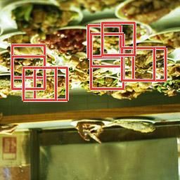
Max-Margin Multiple-Instance Dictionary Learning

       Table 1. Classification accuracy and number of codewords used of different methods on 15 Scene dataset.
                                   Methods                 Accuracy (%) Number of codewords
                         Object Bank (Li et al., 2010)         80.90                 2400
                    Lazebnik et al.(Lazebnik et al., 2006)  81.10±0.30                200
                         Yang et al.(Yang et al., 2009)     80.40±0.45               1024
                     Kernel Descriptors (Bo et al., 2010)  86.70±0.40                1000
                                     Ours                   86.35±0.45                165

Table 2. Classification accuracy on MIT 67 Indoor dataset.   Table 3. Classification accuracy on UIUC Sports dataset.
                                                                             Methods               Accuracy (%)
                 Methods                      Accuracy(%)         Li et al.(Li & Fei-Fei, 2007)        73.4
 ROI+Gist (Quattoni & A.Torralba, 2009)           26.5            Wu et al.(Wu & Rehg, 2009)           84.3
       MM-scene (Zhu et al., 2010)                28.0            Object Bank (Li et al., 2010)        76.3
       Centrist (Wu & Rehg, 2011)                 36.9            SPMSM (Kwitt et al., 2012)           83.0
      Object Bank (Li et al., 2010)               37.6           LPR (Sadeghi & Tappen, 2012)         86.25
    DPM (Pandey & Lazebnik, 2011)                 30.4                         Ours                88.47±2.32
        RBoW (Parizi et al., 2012)               37.93
    Disc. Patches (Singh et al., 2012)            38.1
       SPMSM (Kwitt et al., 2012)                 44.0
     LPR (Sadeghi & Tappen, 2012)                44.84       they combine Discriminative Patches with DPM, Gist-
                  Ours                           50.15
                                                             color, and SP and obtained a classification accuracy of
                                                             49.4%. Our much better performance indicates the
                                                             efficiency and effectiveness of MMDL.
 1. MMDL can naturally learn a metric to take the
    advantage of multiple features.
                                                             5.3. UIUC Sports Image Classification
 2. The max-margin formulation leads to very com-
    pact code for image representation and very com-         In this experiment, we report the performance result
    petitive performance. It is clearly better than the      of event recognition in the UIUC Sports dataset. For
    naive solution.                                          each event category, we only learn 11 different G-
                                                             codes. This results in 88 codewords in total for image
5.2. Indoor Scene Image Classification                       representation. However, our performance is consis-
                                                             tently better than object bank (requires detailed hu-
In the experiment on MIT 67 Indoor dataset, for each         man annotations) and two very recent approaches, L-
of the 67 classes, we learn 11 G-codes, 10 for positive      PR (Sadeghi & Tappen, 2012) and SPMSM (Kwit-
cluster and 1 for negative cluster. Therefore, we have       t et al., 2012) as shown in Table. 3. In addition, a
737 G-codes in total. Fig. 6 shows some cluster models       codebook learning method (Wu & Rehg, 2009) using
learned in buffet and computer-room category. Take           histogram intersection kernel has also been compared.
the computer-room category as an example: cluster 2
corresponds to computers; and cluster 8 corresponds to
desks. Clusters are learned given no more than image
                                                             6. Conclusion
class labels. But it seems that they are very semantic       In this paper, we have proposed a dictionary learning
meaningful.                                                  strategy along the line of multiple instance learning.
Table. 2 summarizes the performances of our method           We demonstrate the effectiveness of our method, which
and some previously published methods. Our perfor-           is able to learn compact codewords and rich semantic
mance is much better than traditional scene recogni-         information.
tion methods, such as (Quattoni & A.Torralba, 2009;
Zhu et al., 2010; Wu & Rehg, 2011). Here we fo-              Acknowledgment: The work was supported by
cus on comparisons with three mid-level image rep-           NSF CAREER award IIS-0844566, NSF award IIS-
resentations, DPM (Pandey & Lazebnik, 2011), R-              1216528, and NIH R01 MH094343. Part of this work
BoW (Parizi et al., 2012), and Discriminative Patch-         was done while the first author was an intern at Mi-
es (Singh et al., 2012). DPM, RBoW and our methods           crosoft Research Asia. It is also in part supported
have used labels of training images for learning. Dis-       by the National Natural Science Foundation of Chi-
criminative Patches method learns mid-level represen-        na (NSFC) Grants 60903096, 61173120 and 61222308.
tation in an unsupervised way. In (Singh et al., 2012),      Xinggang Wang was supported by Microsoft Research
Max-Margin Multiple-Instance Dictionary Learning

     buffet
    cluster 1

    buffet
   cluster 9

computer-room
   cluster 2

computer-room
   cluster 8

Figure 6. Some meaningful clusters learned by MMDL for different categories. Each row illustrates a cluster model: red
rectangles shows positions of G-code classifier fired where SVM function value is bigger than zero.

Asia Fellowship 2012. We thank Jun Zhu, Liwei Wang,           Dollár, P., Babenko, B., Belongie, S., Perona, P., and Tu,
and Quannan Li for helpful discussions.                         Z. Multiple component learning for object detection.
                                                                ECCV, pp. 211–224, 2008.

References                                                    Duda, R., Hart, P., and Stork, D. Pattern Classification
                                                                and Scene Analysis. John Wiley and Sons, 2000.
Andrews, S., Tsochantaridis, I., and Hofmann, T. Support
  vector machines for multiple-instance learning. NIPS,       Fan, Rong-En, Chang, Kai-Wei, Hsieh, Cho-Jui, Wang,
  15:561–568, 2002.                                             Xiang-Rui, and Lin, Chih-Jen. LIBLINEAR: A library
                                                                for large linear classification. Journal of Machine Learn-
Blei, David M., Ng, Andrew Y., and Jordan, Michael I.           ing Research, 9:1871–1874, 2008.
  Latent dirichlet allocation. J. of Machine Learning Res.,
  3:993–1022, 2003.                                           Farhadi, A., Endres, I., Hoiem, D., and Forsyth, D. De-
                                                                scribing objects by their attributes. In CVPR, pp. 1778–
Bo, L., Ren, X., and Fox, D. Kernel descriptors for visual      1785, 2009.
  recognition. NIPS, 7, 2010.
                                                              Fei-Fei, L. and Perona, P. A bayesian hierarchical model
Bourdev, Lubomir and Malik, Jitendra. Poselets: Body            for learning natural scene categories. In CVPR, 2005.
  part detectors trained using 3d human pose annotations.
  In ICCV, 2009.                                              Felzenszwalb, P.F., Girshick, R.B., McAllester, D., and
                                                                Ramanan, D. Object detection with discriminative-
Chatfield, K., Lempitsky, V., Vedaldi, A., and Zisserman,       ly trained part-based models. IEEE Transactions on
  A. The devil is in the details: an evaluation of recent       Pattern Analysis and Machine Intelligence, 32(9):1627–
  feature encoding methods. In BMVC, 2011.                      1645, 2010.

Crammer, K. and Singer, Y. On the algorithmic implemen-       Hinton, G. E., Osindero, S., and Teh, Y. W. A fast learning
  tation of multiclass kernel-based vector machines. The        algorithm for deep belief nets. Neural Computation, 18
  Journal of Machine Learning Research, 2:265–292, 2002.        (7):1527–1554, 2006.

Dietterich, T.G., Lathrop, R.H., and Lozano-Perez, T.         Jiang, Z., Zhang, G., and Davis, L.S. Submodular dictio-
  Solving the multiple-instance problem with axis parallel       nary learning for sparse coding. In CVPR, pp. 3418–
  rectangles. Artificial Intelligence, 89:31–71, 1997.           3425. IEEE, 2012.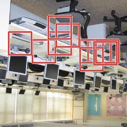
Max-Margin Multiple-Instance Dictionary Learning

Jurie, F. and Triggs, B. Creating efficient codebooks for       Sadeghi, F. and Tappen, M.F. Latent pyramidal regions
  visual recognition. In ICCV, pp. 604–610, 2005.                 for recognizing scenes. In ECCV, 2012.

Kwitt, R., Vasconcelos, N., and Rasiwasia, N. Scene recog-      Serre, Thomas and Poggio, Tomaso. A neuromorphic ap-
 nition on the semantic manifold. In ECCV, 2012.                  proach to computer vision. Commun. ACM, 53(10):54–
                                                                  61, 2010.
Lazebnik, S. and Raginsky, M. Supervised learning of
  quantizer codebooks by information loss minimization.         Singh, Saurabh, Gupta, Abhinav, and Efros, Alexei A. Un-
  IEEE Tran. PAMI, 31:1294–1309, 2009.                            supervised discovery of mid-level discriminative patches.
                                                                  In ECCV, 2012.
Lazebnik, S., Schmid, C., and Ponce, J. Beyond bags of fea-
  tures: Spatial pyramid matching for recognizing natural       Torresani, L., Szummer, M., and Fitzgibbon, A. Efficient
  scene categories. In CVPR, volume 2, pp. 2169–2178,             object category recognition using classemes. ECCV, pp.
  2006.                                                           776–789, 2010.
                                                                Vedaldi, A. and Fulkerson, B. VLFeat: An open and
LeCun, Y., Huang, F., and Bottou, L. Learning methods             portable library of computer vision algorithms, 2008.
  for generic object recognition with invariance to pose
  and lighting. In Proc. of CVPR, June 2004.                    Wang, J., Yang, J., Yu, K., Lv, F., Huang, T., and Gong,
                                                                 Y. Locality-constrained linear coding for image classifi-
Li, L.J. and Fei-Fei, L. What, where and who? classifying        cation. In CVPR, pp. 3360–3367, 2010.
   events by scene and object recognition. In ICCV, 2007.
                                                                Winn, J., Criminisi, A., and Minka, T. Object categoriza-
Li, L.J., Su, H., Xing, E.P., and Fei-Fei, L. Object bank:       tion by learned universal visual dictionary. In ICCV,
   A high-level image representation for scene classification    volume 2, pp. 1800–1807, 2005.
   and semantic feature sparsification. NIPS, 24, 2010.
                                                                Wu, J. and Rehg, J.M. Beyond the euclidean distance:
Lowe, D. G. Distinctive image features from scale-invariant      Creating effective visual codebooks using the histogram
  keypoints. Int’l J. of Comp. Vis., 60(2):91–110, 2004.         intersection kernel. In ICCV, pp. 630–637, 2009.

Mairal, J., Bach, F., and Ponce, J. Task-driven dictionary      Wu, J. and Rehg, J.M. Centrist: A visual descrip-
 learning. arXiv preprint arXiv:1009.5358, 2010.                 tor for scene categorization. IEEE Transactions on
                                                                 Pattern Analysis and Machine Intelligence, 33(8):1489–
Moosmann, F., Triggs, B., and Jurie, F. Fast discrim-            1501, 2011.
 inative visual codebooks using randomized clustering
 forests. In NIPS, pp. 985–992, 2006.                           Xu, Y., Zhu, J.Y., Chang, E., and Tu, Z. Multiple clus-
                                                                  tered instance learning for histopathology cancer image
Moosmann, Frank, Nowak, Eric, and Jurie, Frédéric. Ran-         classification, segmentation and clustering. In CVPR,
 domized clustering forests for image classification. IEEE        pp. 964–971, 2012.
 Trans. Pattern Anal. Mach. Intell., 30(9):1632–1646,
 2008.                                                          Yang, J., Yu, K., Gong, Y., and Huang, T. Linear spatial
                                                                  pyramid matching using sparse coding for image classi-
Ojala, T., Pietikäinen, M., and Harwood, D. A compara-           fication. In CVPR, pp. 1794–1801, 2009.
  tive study of texture measures with classification based      Yang, J., Yu, K., and Huang, T. Supervised translation-
  on feature distributions. Pattern Recognition, 29:51–59,        invariant sparse coding. In CVPR, pp. 3517–3524. IEEE,
  1996.                                                           2010.
Oliva, Aude and Torralba, Antonio. Modeling the shape of        Yang, L., Jin, R., Sukthankar, R., and Jurie, F. Unifying
  the scene: A holistic representation of the spatial enve-       discriminative visual codebook generation with classifi-
  lope. International Journal of Computer Vision, 42(3):          er training for object category recognition. In Proc. of
  145–175, 2001.                                                  CVPR, 2008.
Pandey, M. and Lazebnik, S. Scene recognition and weak-         Zhang, Dan, Wang, Fei, Si, Luo, and Li, Tao. M3ic: maxi-
  ly supervised object localization with deformable part-         mum margin multiple instance clustering. In IJCAI, pp.
  based models. In ICCV, pp. 1307–1314. IEEE, 2011.               1339–1344, 2009.
Parikh, D. and Grauman, K. Relative attributes. In ICCV,        Zhang, Min-Ling and Zhou, Zhi-Hua. M3miml: A max-
  pp. 503–510, 2011.                                              imum margin method for multi-instance multi-label
                                                                  learning. In ICDM, pp. 688–697, 2008.
Parizi, S.N., Oberlin, J.G., and Felzenszwalb, P.F. Recon-
  figurable models for scene recognition. In CVPR, pp.          Zhu, J., Li, L.J., Fei-Fei, L., and Xing, E.P. Large margin
  2775–2782. IEEE, 2012.                                          learning of upstream scene understanding models. NIPS,
                                                                  24, 2010.
Pechyony, D. and Vapnik, V. On the theory of learning
  with privileged information. In NIPS, 2010.                   Zhu, J., Zou, W., Yang, X., Zhang, R., Zhou, Q., and
                                                                  Zhang, W. Image Classification by Hierarchical Spatial
Quattoni, A. and A.Torralba. Recognizing indoor scenes.           Pooling with Partial Least Squares Analysis. In British
  In CVPR, 2009.                                                  Machine Vision Conference, 2012.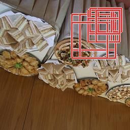
You can also read