Optimizing 1-Nearest Prototype Classifiers
←
→
Page content transcription
If your browser does not render page correctly, please read the page content below
Optimizing 1-Nearest Prototype Classifiers

             Paul Wohlhart, Martin Köstinger, Michael Donoser, Peter M. Roth, Horst Bischof
            Institute for Computer Vision and Graphics, Graz University of Technology, Austria
                        {wohlhart,koestinger,donoser,pmroth,bischof}@icg.tugraz.at

                         Abstract                                    Since powerful classifiers such as non-linear kernel Sup-
                                                                 port Vector Machines (SVMs) have shown excellent perfor-
   The development of complex, powerful classifiers and          mance in diverse computer vision applications it seems to
their constant improvement have contributed much to the          be a natural choice to directly apply them to the available
progress in many fields of computer vision. However, the         large-scale datasets. Unfortunately, such non-linear kernel
trend towards large scale datasets revived the interest in       classifiers are in general computationally too expensive for
simpler classifiers to reduce runtime. Simple nearest neigh-     applications in large-scale settings. For this reason, explicit
bor classifiers have several beneficial properties, such as      feature mappings have been proposed that approximate spe-
low complexity and inherent multi-class handling, however,       cific kernels in a linear manner. For example in [11] an
they have a runtime linear in the size of the database. Re-      approximation of the popular intersection kernel was de-
cent related work represents data samples by assigning           scribed. This approach was then generalized to the set of
them to a set of prototypes that partition the input feature     homogeneous, additive kernels (including the intersection
space and afterwards applies linear classifiers on top of        and chi-squared kernel) in [16]. Nevertheless, not all ker-
this representation to approximate decision boundaries lo-       nels can be approximated in such a manner. Furthermore,
cally linear. In this paper, we go a step beyond these ap-       optimal classification decision boundaries do not necessar-
proaches and purely focus on 1-nearest prototype classifi-       ily exhibit the structure as defined by a kernel.
cation, where we propose a novel algorithm for deriving op-         On the contrary, linear classifiers are fast enough to be
timal prototypes in a discriminative manner from the train-      applicable in large-scale scenarios, especially due to recent
ing samples. Our method is implicitly multi-class capable,       developments in efficiently solving the corresponding opti-
parameter free, avoids noise overfitting and, since during       mization problem. For example, in [14] a stochastic gra-
testing only comparisons to the derived prototypes are re-       dient descent approach for solving the optimization prob-
quired, highly efficient. Experiments demonstrate that we        lem of linear SVMs was introduced, where the total run-
are able to outperform related locally linear methods, while     time does not directly depend on the size of the training set.
even getting close to the results of more complex classifiers.   The approach also extends to non-linear kernels by solely
                                                                 working on the primal, nevertheless, in these cases runtime
                                                                 scales linearly with training set size.
1. Introduction
                                                                    Unfortunately, a global, linear model is seldom power-
    Over the last decade we have seen an impressive progress     ful enough to separate the data. For this reason, locally
in important fields of computer vision like image clas-          linear classifiers have been attracting a lot of attention re-
sification and object detection, which is mainly a result        cently. The core idea of these methods is to define the op-
of developments in supervised machine learning and the           timal decision boundary by locally linear approximations
steadily growing amount of available training data. Large-       that are defined on prototypes. These prototypes (or anchor
scale datasets for effectively training classifiers have al-     points) reside in the same space as the input data points and
ready proven to be quite beneficial in several contexts. For     the classifier is then trained and evaluated in the context of
example, the seminal work on using random forest classi-         a local neighborhood around them. A recent example for
fiers on single depth images for estimating human poses          such a classifier is the Locally Linear SVM (LL-SVM) pro-
(Microsoft KinectTM ) [15] heavily exploits a huge set of        posed in [9], where the non-linear decision boundary is ap-
synthetically generated human pose depth images during           proximated with many linear SVMs. Data points are soft-
training. Also, the recent advances on the PASCAL visual         assigned to anchor points identified by k-means and SVM
object recognition challenge can largely be attributed to the    parameters are jointly learned in a common optimization
steady increase in training database sizes [19].                 problem. This can be solved by stochastic gradient descent,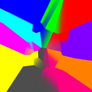
with the same convergence guarantees as for standard, lin-        tion based on max-margin principles was introduced and it
ear SVMs. In a related work a multi-class classifier denoted      is demonstrated that the original LVQ [8] represents a spe-
as Parametric Nearest Neighbor (PNN) and its ensemble ex-         cific instance of the proposed framework. Remarkably, the
tension (EPNN) was proposed [18]. The core idea is to em-         authors demonstrate that prototype based classification is
bed data points into a new feature space, again defined by        even able to outperform nearest neighbor classification us-
soft assignments to prototypes, and to learn a linear max-        ing all training data due to improved generalization proper-
margin classifier on this new representation. An iterative        ties caused by a reduction of over-fitting to noise.
method is introduced, that alternately optimizes the proto-           In this paper, we address large-scale classification by a
types and then the classifier parameters. Interestingly, rea-     prototype based nearest neighbor approach. We aim to go
sonable performance is only obtained when the optimiza-           beyond the most related methods of [9, 18], where local
tion is not run until convergence and an ensemble of such         codings based on prototypes are used in a subsequently ap-
base classifiers is formed.                                       plied classifier, by completely focusing on the most simple
    The necessity for large-scale classification has in gen-      variant: a 1-nearest neighbor (NN) algorithm. Instead of
eral led to a comeback of non-parametric classifiers like         considering all N training samples in the 1-NN algorithm
the nearest neighbor algorithm. Nearest neighbor classi-          as done in [8, 13, 3], we aim at discriminatively deriving a
fiers have several interesting properties: (a) they allow im-     small, optimal set of P prototypes with P  N and base
plicit multi-class decisions and naturally handle even a huge     our classification decision completely on the single label of
number of classes, (b) they, in general, avoid overfitting,       the nearest neighbor within this prototype set.
which is important to obtain reasonable classification ac-            To reach this goal, we present a differentiable probabilis-
curacy and (c) they do not require any training effort. For       tic relaxation of 1-NN classification, based on soft assign-
example, in [1] it was shown that for Bag-of-words based          ments of samples to prototypes, that can be optimized us-
image classification, simple adaptations in the visual word       ing gradient descent. It has one parameter controlling the
quantization and in the image-to-image distance calculation       softness of the assignment. Letting this parameter go to in-
are sufficient to achieve state-of-the-art results using a sim-   finity leads to pure 1-NN classification. Thus, in contrast
ple nearest neighbor method as subsequent classifier.             to related methods, we can provide discriminative proto-
    Nearest neighbor classification especially shows promis-      types directly optimized for subsequent pure 1-NN classi-
ing performance in combination with metric learning (e.g.,        fication, by gradually decreasing the softness of the assign-
[17]), where the assignment to the nearest neighbors is           ment while optimizing the prototypes.
based on a Mahalanobis distance metric instead of the com-            Our method exhibits the same advantages as standard
mon Euclidean distance. In general, such methods aim at           prototype based nearest neighbor classification: (a) It is pa-
improving the nearest neighbor classification, e.g., by en-       rameter free, (b) it is implicitly able to handle large numbers
suring that all k-nearest neighbors belong to the same class,     of classes, (c) it avoids over-fitting to noise and generalizes
whereas examples from differing classes should be sepa-           well to previously unseen samples as also demonstrated in
rated by a large margin. In such a way, these methods are         the experiments, and (d) it has very low computational costs
a counterpart to max-margin classifiers like SVMs, where          during testing, since only distances to the P prototypes have
nearest neighbor assignments replace the weighted sum of          to be evaluated (with possible further improvements using
(kernelized) distances to support vectors.                        fast nearest neighbor assignment methods like KD-trees).
    An interesting way to further reduce the complexity of        In thorough experiments, we demonstrate that our discrim-
nearest neighbor classifiers is to constrain the analysis to      inatively learned prototypes consistently outperform the k-
selected prototypes, instead of considering all training data     means baseline, even with very low numbers of prototypes.
samples during testing. Obviously, performance is heav-           Furthermore, we show that already a very small number of
ily depending on a reasonable selection of the prototypes.        prototypes is sufficient to obtain reasonable classification
Finding optimal prototypes from labeled data has a long his-      accuracy on several datasets. Our method naturally allows
tory, where methods are in general referred to as Learning        to integrate learned Mahalanobis metrics like [17]. How-
Vector Quantization (LVQ). This field was initiated by the        ever, we show that by learning the prototypes in the pro-
seminal work of [8], where a heuristic was used to move           posed discriminative manner, learning Mahalanobis metrics
prototypes close to training samples of the same class and        becomes less important.
away from other classes. The method was later adapted                 The outline of the paper is as follows. We first show
in [13], where the problem was formulated as an optimiza-         in Section 2, how to relax the 1-nearest neighbor classifi-
tion problem maximizing the likelihood ratio between the          cation to a soft-max variant, which then allows to find the
probability of correct classification and the total probabil-     prototypes using gradient descent by minimizing the empir-
ity in a Gaussian Mixture Model (each prototype is repre-         ical risk of misclassification over the entire training dataset.
sented as a Gaussian). In [3] a supervised vector quantiza-       We derive formulations for the exponential and the hinge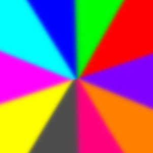
loss, and discuss possible influences on the results. Sec-       where d? is a distance and typically chosen to be the squared
tion 3 gives illustrative results on toy examples, as well as    Euclidean distance:
a thorough comparison to state-of-the-art on three standard
                                                                                                                  2
classification datasets.                                                        deuc (x1 , x2 )   =    ||x1 − x2 || .          (5)

2. Method                                                           Inspired by the recent developments in metric learning,
                                                                 we also consider learned Mahalanobis distance metrics M
   Given a training set T with labeled samples (xi , yi ),       to define the distances between samples:
where xi ∈ Rd and yi ∈ {−1, 1}, the goal is to define
a classifier f (x) = y that correctly classifies test sam-             dmetric (x1 , x2 )   =
                                                                                                            T
                                                                                                  (x1 − x2 ) M (x1 − x2 ) .    (6)
ples from the same distribution. As discussed before, to
reduce the model complexity and the test time, our pro-          In practice, we do not use dmetric directly, but decompose
posed classifier is a prototype based 1-nearest neighbor al-     M into M = LT L and project the input features x onto L
gorithm. We aim at deriving discriminative, labeled pro-         by x̂i = Lxi . In this way, we can again use the Euclidean
totypes (pj , θj ) ∈ P, pj ∈ Rd , θj ∈ {−1, 1}, that are         distance to measure distances in the transformed space.
optimized for simple 1-nearest neighbor classification:
                                                                 2.2. Choosing γ
        f (x) = θk , where k = arg min ||x − pj || .      (1)
                                         j                           Notice, if γ is set to infinity (or a very high value in prac-
                                                                 tice) when calculating the weights in Eq. (3), every sample
    To get an optimal classifier, the prototypes pj must be
                                                                 gets assigned a weight of 1 only for its closest prototype.
arranged such as to minimize the empirical risk of misclas-
                                                                 Thus, in the soft-max classifier shown in Eq. (2) the sample
sification. Thus, we formulate the optimization of the pro-
                                                                 is directly assigned the label of its closest prototype, exactly
totypes as a gradient descent on a loss function over the
                                                                 as in the original 1-NN formulation. With lower values of
training examples. Since the original formulation of 1-NN
                                                                 γ more weight is given to the next closest prototypes and
shown in Eq. (1) is not differentiable, we relax the hard as-
                                                                 more distant interactions are established, until for γ = 0 all
signment of samples to prototypes to a soft-max formula-
                                                                 locality vanishes and the result of a classification is just the
tion over sample similarities (i.e., soft-min over distances).
                                                                 prior distribution of the training labels. This indicates that
The following sections describe the setup of the relaxed
                                                                 the choice of γ essentially influences the results.
classifier.
                                                                     We would like to emphasize that the soft-max classifier
2.1. Classifier                                                  defined in the previous section is only used as a surrogate
                                                                 for our finally applied classifier. The discriminatively de-
    Given the set of optimized prototypes, we define the clas-   rived prototypes are then supposed to be used in 1-NN clas-
sifier as the weighted sum of the prototypes’ labels:            sification, as in Eq. (1). If we were sacrificing the benefit
                              |P|
                                                                 of the simple 1-NN classification and looking for an opti-
                              X                                  mal soft-max classifier as defined in Eq. (2), we would also
                    f (x) =         θj wj (x) .           (2)
                              j=1
                                                                 need to optimize for γ.
                                                                     However, for our goal of defining an effective 1-NN clas-
    The weights are defined by a soft-max over the similari-     sifier, we consider an iterative approach, where we start with
ties between input sample x and prototypes pj :                  a low value for γ. In this way, we allow more than one pro-
                                                                 totype to have influence on a sample, and thus vice versa,
                                             γ
                           s(x, pj )                             let each sample have influence on more than one prototype.
                wj (x) = P|P|            ,                (3)
                                       γ                         For the current γ-value, we derive optimal prototypes using
                          k=1 s(x, pk )
                                                                 a gradient descent approach as outlined in the next section.
where s(x1 , x2 ) is the similarity of samples x1 and x2 ,       Then, in each iteration, we gradually increase γ and again
and γ controls the degree of softness in the assignment,         optimize the prototypes, until virtually all samples are only
which will be discussed in Sec. 2.2. The weights for all         influenced by a single prototype, arriving at pure 1-NN clas-
prototypes for one training sample sum up to 1, i.e., ∀x :       sification. In such a way, we can avoid local minima result-
P|P|
                                                                 ing from overfitting.
  j=1 wj (x) = 1, resulting in a probabilistic output for the
overall classifier.                                                  In practice, we initialize γ such that the difference be-
   The similarity of two samples is defined as the negative      tween the highest and the second highest prototype weight
exponential of the distance between the samples:                 is less than 0.5 for at least 80% of the training samples. We
                                                                 then increase γ until for every training sample there is sig-
            s(x1 , x2 )   =   exp(−d? (x1 , x2 )) ,       (4)    nificant weight for only a single prototype (i.e., the sum over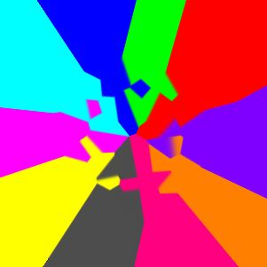
all other weights drops below a very low threshold), but cal-         Total Loss
culation of the weights is still numerically stable. As inter-
                                                                                                         |T |
mediate steps we interpolate 10 values between the lowest                            ∂L(T , ∆? ) X ∂∆? (f (xi ), yi )
                                                                                                =                                         (10)
and the highest value on a logarithmic scale.                                           ∂pl             ∂pl
                                                                                                  i=1

2.3. Empirical loss over training data                                Loss Functions
    In order to optimize the prototypes with gradient descent,             ∂∆exp (f (xi ), yi )                        ∂f (xi )
we need to design a derivable loss function, measuring the                                      = −yi exp(−yi f (xi ))                    (11)
                                                                                  ∂pl                                   ∂pl
quality of the output of the current probabilistic classifier
setup. Given the definition of the classifier, the loss over all
training samples is defined by                                                                     (
                                                                        ∂∆hinge (f (xi ), yi )         −yi ∂f∂p
                                                                                                              (xi )
                                                                                                                         if yi f (xi ) < δ
                                                                                               =                l
                                                                                                                                           (12)
                              |T |                                             ∂pl                     0                 otherwise
                              X
              L(T , ∆? ) =           ∆? (f (xi ), yi ) ,      (7)
                              i=1                                     Classifier
where ∆? is a function measuring the loss of the classifi-                                                |P|
                                                                                          ∂f (xi ) X ∂wj (xi )
cation outcome. In particular, we apply two types of loss                                         =     θj                                (13)
                                                                                           ∂pl             ∂pl
functions, namely the exponential loss                                                              j=1

             ∆exp (f (xi ), yi ) = exp (−yi f (xi ))          (8)     Weights

                                                                                   ∂wj (xi )   γwj (xi ) ∂s(xi , pj )
and the hinge loss                                                                           =                          −                 (14)
                                                                                     ∂pl       s(xi , pj )      ∂pl
         ∆hinge (f (xi ), yi ) = max(0, δ − yi f (xi )) ,     (9)                              γwj (xi )            ∂s(xi , pl )
                                                                                             −             wl (xi )                       (15)
                                                                                               s(xi , pl )             ∂pl
which is more robust to outliers, where with δ the margin
can be adjusted. Due to the probabilistic formulation of our          Similarities
classifier, an output of more than 0.5 for the correct class                        ∂s(xi , pj )                ∂d? (xi , pj )
means that no other class can have a larger value and δ can                                      = −s(xi , pj )                           (16)
                                                                                       ∂pl                          ∂pl
be adjusted to preserve a margin but not to overfit. A hinge
loss formulation was also used in [18].                               Distances
                                                                                                      (
2.4. Derivatives w.r.t. prototypes                                               ∂deuc (xi , pj )         −2(xi − pl ) if l = j
                                                                                                  =                                       (17)
   In order to perform the gradient descent, we need the                             ∂pl                  0            else
derivatives w.r.t. the prototype vectors. Since we have dif-
ferent choices at some parts of the formulation, we show the          Using the Euclidean distance d? = deuc , the derivation of
partial derivative for each component individually in Fig-            the classifier w.r.t. the prototypes thus reduces to
ure 1.                                                                       ∂f (xi )
                                                                                      = 2γwl (xi )(xi − pl ) (θl − f (xi )) .             (18)
2.5. Multiclass                                                               ∂pl
                                                                     Figure 1. Partial derivatives for each individual part of the classifi-
    For notational convenience we have only discussed bi-            cation loss w.r.t prototype locations, as needed for the optimization
nary classification up to this point. In the case of multi-          with gradient descent.
class classification tasks with C classes we adopt a lifted
formulation and extend training and prototype labels to vec-
                                                                        The multi-class loss is then defined as the sum over the
tors yi , θj ∈ {−1, 1}C (i.e., yi = (yi,1 , . . . , yi,C )), where
                                                                     losses for each individual class:
yi,ci = 1 for a sample xi of class ci and all other entries
are −1. The overall classifier then takes the max over the                                             C
                                                                                                       X
predictions for each class                                                            L(T , ∆? ) =              Lc (T , ∆? ) ,          (20)
                                                                                                       c=1

                   F (x) = arg max fc (x) ,                  (19)                         P|T |
                                                                     where Lc (T , ∆? ) = i=1 ∆? (fc (xi ), yi,c ).
                                     c
                 P|P|                                                   We also considered a formulation that optimizes the mar-
where fc (x) =       j=1 θj,c wj (x).                                gin between the classification of the target class and the out-
put for the most confident non-target class for each sample, the initial k-means clustering, is drastically reduced. The
instead of the output for all classes: hinge loss smoothes the decision boundary more than the
exponential loss, where for higher values of γ the deci-
|T |
X sion boundaries tend to fit more around single samples that
L(T , ∆? ) = ∆? (fci (xi ), yi,ci )+max ∆? (fcj (xi ), yi,cj ) . are scattered into areas that are more densely populated by
cj 6=ci
i=1 samples from differing classes. Note also the very differ-
(21)
ent configuration of the finally obtained prototypes for the
Such a formulation was chosen in [18]. However, although
two different loss functions. Generally, with the hinge loss
this formulation yields meaningful results on toy examples,
the prototypes tend to be grouped together to more generic
it consistently produced considerably worse result than the
locations, whereas with the exponential loss prototypes dis-
formulation in Eq. (20) on real world data, which is why we
tribute more to also capture instances in low density areas.
excluded it from further considerations.
Whether this is beneficial depends on the distribution and
especially separability of the data. The difference is also
3. Experiments reflected in the performance plots, which show steadily in-
We first outline characteristics of our proposed method creased training accuracy for increasing γ values in both
for selecting optimal prototypes for 1-NN classification on cases, but a slight breakdown in the test accuracy for the
two toy examples in Section 3.1. Then, Section 3.2 pro- exponential loss. However, the performance is still better
vides a thorough quantitative comparison of our algorithm compared to the k-means initialization.
to related work on real world computer vision datasets.
3.2. Image classification
In all experiments, we initialize our method using proto-
types defined by applying k-means clustering for each class We evaluate our method on three widely used classifica-
individually. We also experimented with taking a random tion datasets, each providing sufficient training samples per
subset of the training data as initial prototypes. This usu- class, such that a reduction to a small set of discriminative
ally leads to similar results, but is more susceptible to local prototypes really pays off.
minima, especially if modes of the distribution do not get The first database is USPS [7], which contains 7291
a nearby, initial prototype. In contrast, k-means initializa- training and 2007 test gray-scale images of the digits ’0’
tion ensures a certain coverage of the training sample distri- to ’9’, stored with a resolution of 16 × 16 pixels. Addition-
bution. Starting from the k-means initialization, we apply ally, we test on the LETTER database [6], which contains
our iterative prototype updating as described in the previ- 16000 training and 4000 testing images of the letters ’A’ to
ous section using the non-linear conjugate gradient descent ’Z’. Each of them is represented by a 16 dimensional fea-
method (ncg) from the Poblano Toolbox [4]. Our final clas- ture vector. Finally, we also evaluate on MNIST [10]. It
sifier is then defined by using the obtained prototypes in a contains 60000 training and 10000 test gray-scale images
1-NN assignment strategy, as defined in Eq. (1). of the digits ’0’ to ’9’ with a resolution of 28 × 28 pixels.
For MNIST we took the publicly available data from [12]
3.1. Illustrative toy examples and LETTER and USPS are taken from [9].
We illustrate how prototypes evolve during our optimiza- We list classification errors on these three datasets for all
tion for two 2D toy examples, namely a dataset consisting of variants of our method in comparison to related work in Ta-
three classes with multimodal distributions and a dataset of ble 1. Our proposed Nearest Prototype Classifier (NPC)
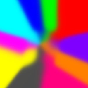
10 classes with regular structure. Figures 2 and 3 show pro- with exponential loss is denoted by NPC-e and with hinge
totypes and the consequently emerging decision surfaces for loss NPC-h. We show results for different numbers k of
1-nearest neighbor classification using either the exponen- prototypes per class. For example, a value of k = 15 means
tial or the hinge loss during our iterative prototype update a reduction to 0.25% of the number of available training
method. Results are shown starting from k-means cluster- samples for MNIST, 2.06% for USPS and 2.4% for LET-
ing and updating until convergence (Fig. 2(a)-2(e) and 3(a)- TER. Table 1 further shows results if using a learned global
3(e)). Additionally, we illustrate classification performance Mahanalobis metric obtained by applying LMNN [17] in-
on train and test data during optimization (Fig. 2(f)-(g) and stead of standard Euclidean distances. Additionally, the ta-
3(f)-(g)), where the x-axis represents the value of γ used to ble outlines results for the most related state-of-the-art ap-
optimize the prototypes in the current iteration of the algo- proaches [9, 18], as well as linear and RBF-kernel SVMs.
rithm, the y-axis represents values of γ used in the soft-max
over similarities, and the height of the mesh reflects the cor- Discussion As can be seen in Table 1 our proposed Near-
responding classification accuracy. est Prototype Classifier (NPC) achieves highly competitive
Note that the decision surfaces become much smoother error rates in comparison to related state-of-the-art methods
during prototype evolution and that overfitting, prevalent for although solely relying on simple prototype based 1-nearest(a) init k-means (b) exp loss, iteration 1 (c) exp loss, final (d) hinge loss, iteration 1 (e) hinge loss, final
0.98 1 0.98
1
0.96 0.96
0.98
0.98 0.94 0.94
0.96 0.92 0.96 0.92
156.25 156.25 156.25 156.25
89.74 156.25 89.74 156.25 89.74 156.25 89.74 156.25
gam51.5429.6 68.01 gam51.5429.6 68.01 gam51.5429.6 68.01 gam51.5429.6 68.01
ma 29.6 ma 29.6 ma 29.6 ma 29.6
17 12.89 a o pt 17 12.89 a o pt 17 12.89 a o pt 17 12.89 a o pt
eva m eva m eva m eva m
l 9.77 init gam l 9.77 init gam l 9.77 init gam l 9.77 init gam
(f) train (left) and test (right) accuracy, exp loss (g) train (left) and test (right) accuracy, hinge loss
Figure 2. Evolution of prototypes during learning on a 2D toy example with 3 classes. Crosses denote samples, circles are prototypes.
(a) init, k-means (b) exp loss, iteration 1 (c) exp loss, final (d) hinge loss, iteration 1 (e) hinge loss, final
0.8 0.82 0.8
0.8 0.8
0.75 0.75
0.75 0.78
0.7 0.76 0.7
156.25 156.25 156.25 156.25
78.13 156.25 78.13 156.25 78.13 156.25 78.13 156.25
gam39.06 55.24 gam39.06 55.24 gam39.06 55.24 gam39.06 55.24
ma 19.539.77 19.53
o pt ma 19.539.77 19.53
o pt ma 19.539.77 19.53
o pt ma 19.539.77 19.53
opt
eva 6.91 m a eva 6.91 ma eva 6.91 m a eva 6.91 m a
l 4.88 init gam l 4.88 init gam l 4.88 init gam l 4.88 init gam
(f) train (left) and test (right) accuracy, exp loss (g) train (left) and test (right) accuracy, hinge loss
Figure 3. Same as in Figure 2 for a 10 class toy example. Each of the classes if defined by a single Gaussian. However the different
Gaussians overlap significantly, such that samples of individual classes get scattered into the area of the neighboring ones.k dist method USPS Letter MNIST ber of prototypes, it is more important to better fit to all the
euc 1-nn 5.08 4.35 2.43 data and overfitting is not so much of an issue.
all
lmnn 1-nn 5.03 2.92 2.38 The effect of using the learned distance metric instead of
euc k-means 7.67 13.75 4.98 Euclidean distances on the classification error varies over
15 the different settings. When using all training samples or
NPC-h 6.23 4.77 2.24
NPC-e 5.38 3.13 2.11 the initial k-means prototypes for the 1-NN classification,
lmnn k-means 6.43 7.40 5.08 the learned metric performs consistently better. Neverthe-
NPC-h 5.73 4.33 2.55 less, if using our discriminatively learned prototypes, the
NPC-e 5.43 3.20 2.22 plain Euclidean distance shows better performance, espe-
euc k-means 6.88 8.23 4.15 cially when the number of learned prototypes is low.
30
NPC-h 5.78 4.33 2.18 Compared to state-of-the-art methods our Nearest
NPC-e 4.98 3.43 1.72 Neighbor Classifier (NPC) delivers highly competitive re-
lmnn k-means 5.98 5.25 4.17 sults. Already with only 15 prototypes, it consistently out-
NPC-h 6.03 3.25 2.32 performs PNN [18], which uses 40 prototypes per class. If
NPC-e 5.33 3.00 1.84 using 50 prototypes, we also improve over the ensemble
euc k-means 6.38 6.55 3.50 version EPNN [18], which uses 800 prototypes (40 per class
50 × 20 weak classifiers). This might be devoted to the more
NPC-h 5.73 4.70 1.89
NPC-e 4.58 3.35 1.57 discriminative nature of our prototypes. In comparison to
lmnn k-means 5.68 4.35 3.48 LL-SVM [9], our method also performs better starting from
NPC-h 5.33 3.95 2.09 k = 15 on USPS and LETTER, and k = 30 for MNIST.
NPC-e 5.28 2.70 1.76 LL-SVM relies on only 100 anchor-points in total (not per
euc k-means 5.23 5.83 3.11 class), but afterwards has to re-evaluate a weighted sum
100 over multiclass SVMs at runtime. Additionally, as shown
NPC-h 5.68 4.37 1.87
NPC-e 4.98 2.85 1.69 in [9], increasing the number of anchor points does not fur-
lmnn k-means 5.43 3.67 2.99 ther improve the results of LL-SVM.
NPC-h 5.78 2.93 1.80 Using our best setup, NPC even gets close to classi-
NPC-e 5.03 2.55 1.61 fication error rates of significantly more complex models
(in terms of test time operations) such as non-linear ker-
40 PNN [18] 7.87 6.59 3.13 nel SVMs. For example, if using 50 prototypes per class,
800 EPNN [18] 4.88 2.90 1.65 Euclidean distances and the exponential loss we reach the
LL-SVM [9] 5.78 5.32 1.85 same performance as a multiclass SVM with RBF kernel
LIBSVM-RBF [2] 4.58 2.12 1.36 on the USPS dataset. On the other two datasets, results are
in close range (using LMNN for the LETTER database).
Linear SVM [5] 8.32 23.63 8.18
Table 1. Comparison of all variants of our method and related work 3.3. Visualization of learned prototypes
on USPS, LETTER and MNIST. All numbers are percentages of Since the input to our classifier is a vector represen-
the classification error. The scores of the best setting per database tation of raw pixel values, it is also possible to visualize
for our algorithm are marked bold.
the learned prototypes in comparison to standard k-means
results. Figure 4 visualizes obtained prototypes for the
neighbor classification. In general, using our learned pro- MNIST dataset, where the discriminatively identified pro-
totypes consistently outperforms the baseline, where proto- totypes are sorted per class in descending importance, ana-
types are defined by k-means clustering results. In several lyzing the sum of weights assigned by the training samples.
cases (e.g. USPS, NPC-e, k=50) our nearest prototype clas- As can be seen, prototypes obtained by k-means clustering
sifier even outperforms 1-NN classification using all train- purely capture generative aspects of different modes of the
ing data samples, although only a few discriminative proto- training data, while our learning approach adds discrimina-
types are considered (e.g., for k = 50 only 7% of the number tive information. For example, around the strokes of the
of training samples of USPS). This clearly demonstrates the individual symbols, as well as in the center of the digit “0”,
ability of our method to identify powerful prototypes in a there must not be other scribbles. Our prototypes reflect this
discriminative manner, while reducing overfitting to noise by featuring negative values in those areas, with the purpose
and improving generalization properties. of increasing the distance to samples of other classes. This
As opposed to the simple 2D toy examples, the exponen- effect is also more pronounced than in [18], most likely be-
tial loss generally performs a bit better than the hinge loss. cause we let the optimization procedure converge to a min-
Apparently, for this kind of data and the relatively low num- imum instead of stopping after a single iteration.References
[1] O. Boiman, E. Shechtman, and M. Irani. In defense
of Nearest-Neighbor based image classification. In Proc.
CVPR, 2008.
[2] C.-C. Chang and C.-J. Lin. LIBSVM: A library for sup-
port vector machines. ACM Trans. on Intelligent Systems
and Technology, 2:27:1–27:27, 2011.
[3] K. Crammer, R. Gilad-bachrach, A. Navot, and N. Tishby.
Margin analysis of the LVQ algorithm. In Advances NIPS,
2002.
[4] D. M. Dunlavy, T. G. Kolda, and E. Acar. Poblano v1.0:
A matlab toolbox for gradient-based optimization. Techni-
cal Report SAND2010-1422, Sandia National Laboratories,
(a) initial prototypes (b) learned discriminative prototypes Albuquerque, NM and Livermore, CA, Mar. 2010.
[5] R.-E. Fan, K.-W. Chang, C.-J. Hsieh, X.-R. Wang, and C.-J.
Figure 4. Samples of some of the prototypes for MNIST (a) ini- Lin. LIBLINEAR: A library for large linear classification.
tialized by k-means and (b) learned with our algorithm. Intensity JMLR, 9:1871–1874, 2008.
levels are scaled such that 0 is grey, lighter pixels are positive and [6] P. W. Frey and D. J. Slate. Letter recognition using holland-
darker negative. style adaptive classifiers. Machine Learning, 6(2):161–182,
1991.
[7] J. Hull. A database for handwritten text recognition research.
4. Conclusion IEEE Trans. on PAMI, 16(5):550–554, May 1994.
[8] T. Kohonen. Self-organization and associative memory.
Prototype based 1-nearest-neighbor (NN) classification Springer-Verlag, New York, 1989.
is one of the simplest and fastest supervised machine learn- [9] L. Ladicky and P. H. S. Torr. Locally linear support vector
ing methods. In this paper we showed that by a probabilistic machines. In Proc. ICML, 2011.
relaxation of the 1-NN classification into a soft-max formu- [10] Y. Lecun, L. Bottou, Y. Bengio, and P. Haffner. Gradient-
lation, we are able to derive optimal prototypes by gradient based learning applied to document recognition. Proceed-
descent in a discriminative manner. Since during testing we ings of the IEEE, 86(11):2278–2324, Nov 1998.
only have to evaluate distances to the few prototypes ob- [11] S. Maji, A. C. Berg, and J. Malik. Classification using inter-
tained, our proposed method is highly efficient, where a fur- section kernel support vector machines is efficient. In Proc.
ther speedup would be possible using approximated nearest CVPR, 2008.
neighbor methods like KD-trees. We further demonstrated [12] D. Ramanan and S. Baker. Local distance functions: A tax-
in the experiments that based on our properly learned set onomy, new algorithms, and an evaluation. IEEE Trans. on
of discriminative prototypes, we can achieve state-of-the- PAMI, 33:794–806, 2011.
art results on challenging datasets, even getting close to the [13] S. Seo and K. Obermayer. Soft learning vector quantization.
Neural Computation, 2002.
performance of significantly more complex classifiers like
[14] S. Shalev-Shwartz, Y. Singer, and N. Srebro. Pegasos: Pri-
non-linear kernel SVMs.
mal estimated sub-gradient solver for svm. In Proc. ICML,
Additionally, we have noticed that, when starting with a 2007.
setting considering more long range interactions, prototypes [15] J. Shotton, A. Fitzgibbon, M. Cook, T. Sharp, M. Finoc-
tend to group together at generic locations. This motivates chio, R. Moore, A. Kipman, and A. Blake. Real-time human
further research on how to start with a rather high number pose recognition in parts from single depth images. In Proc.
of prototypes and select the best ones afterwards. Addition- CVPR, 2011.
ally, it would be interesting to build an anytime algorithm, [16] A. Vedaldi and A. Zisserman. Efficient additive kernels via
by ranking prototypes by importance, such that during test- explicit feature maps. IEEE Trans. on PAMI, 34(3), 2011.
ing the distance calculation could begin at the most impor- [17] K. Weinberger and L. Saul. Distance metric learning for
tant ones and stop after a time budget is used up, always large margin nearest neighbor classification. JMLR, 10:207–
giving the best possible classification up to that point. 244, 2009.
[18] Z. Zhang, P. Sturgess, S. Sengupta, N. Crook, and P. H. S.
Acknowledgement. This work was supported by the Austrian Sci- Torr. Efficient discriminative learning of parametric nearest
ence Foundation (FWF) project Advanced Learning for Tracking neighbor classifiers. In Proc. CVPR, 2012.
and Detection in Medical Workflow Analysis (I535-N23), the Eu- [19] X. Zhu, C. Vondrick, D. Ramanan, and C. C. Fowlkes. Do
ropean Union Seventh Framework Programme (FP7/2007-2013) we need more training data or better models for object detec-
under grant agreement n◦ 601139 (CultAR) and by the Austrian tion? In Proc. BMVC, 2012.
Research Promotion Agency (FFG) project FACTS (832045).You can also read