Media, Pulpit, and Populist Persuasion: Evidence from Father Coughlin - Princeton Economics
←
→
Page content transcription
If your browser does not render page correctly, please read the page content below
Media, Pulpit, and Populist Persuasion:
          Evidence from Father Coughlin
                                    Tianyi Wang∗

                                       Abstract
           New technologies make it easier for charismatic individuals to influ-
       ence others. This paper studies the political impact of the first populist
       radio personality in American history. Father Charles Coughlin blended
       populist demagoguery, anti-Semitism, and fascist sympathies to create
       a hugely popular radio program that attracted tens of millions of listen-
       ers throughout the 1930s. I evaluate the short- and long-term impacts
       of exposure to Father Coughlin’s radio program. Exploiting variation
       in the radio signal strength as a result of topographic factors, I find that
       a one standard deviation increase in exposure to Coughlin’s anti-FDR
       broadcast reduced FDR’s vote share by about two percentage points
       in the 1936 presidential election. Effects were larger in counties with
       more Catholics and persisted after Father Coughlin left the air. An al-
       ternative difference-in-differences strategy exploiting Coughlin’s switch
       in attitude towards FDR during 1932-1936 confirms the results. More-
       over, I find that places more exposed to Coughlin’s broadcast in the late
       1930s were more likely to form a local branch of the pro-Nazi German-
       American Bund, sell fewer war bonds during WWII, and harbor more
       negative feelings towards Jews in the long run.

   Keywords: Mass Media, Charismatic Leader, Religion, Anti-Semitism,
Populism, Great Depression
   ∗
    Department of Economics, University of Pittsburgh, 4901 Wesley W. Posvar Hall, 230
South Bouquet Street Pittsburgh, PA 15260. Email: tianyi.wang@pitt.edu. I am extremely
grateful to Randy Walsh, Osea Giuntella, and Allison Shertzer for their guidance and sup-
port throughout this project. I also thank Stefano DellaVigna, Andreas Ferrara, Matthew
Gentzkow, Taylor Jaworski, Melissa Kearney, Daniel I. Rees, Richard Van Weelden, Eu-
gene White and participants at the Applied Microeconomics Brown Bag at the University
of Pittsburgh, the 2019 Southern Economic Association Annual Conference, the 2019 Eco-
nomic History Association Annual Meeting, the 2019 Cliometric Society Annual Conference,
the 2019 Social Science History Association Annual Meeting, and the 2020 Mountain West
Economic History Conference for their helpful comments and suggestions.

                                            1
1    Introduction
New media and communication technologies make it easier for charismatic
individuals to influence others. The 2016 U.S. presidential election and the
rise of populist leaders across the world heighten the concern that individuals,
through their charisma and media savviness, can manipulate public opinions
for political gain. How and to what extent can charismatic individuals ex-
ploit the media to shape political outcomes? This paper studies the political
impact of the first populist radio personality in American history. Father
Charles Coughlin blended populist demagoguery, anti-Semitism, and fascist
sympathies to create one of the first loyal mass audiences in broadcasting his-
tory, attracting tens of millions of listeners throughout the 1930s (Warren,
1996). This paper assembles a unique data set to evaluate the short- and
long-term impact of exposure to Father Coughlin’s radio program.
      Roman Catholic priest Charles Coughlin embraced radio broadcasting
when radio was a new and rapidly exploding technology during the 1920s. For
the first time one could broadcast to a mass audience over long distances. Ini-
tially airing religious sermons, Father Coughlin switched to broadcast almost
exclusively his opinions on social and economic issues following the onset of
the Great Depression. In a nation mired in its worst economic crisis, Coughlin
became the voice of the people against the nation’s economic and financial
elites. A charismatic orator, Coughlin became seen as the champion of the
common man and referred to as the “Radio Messiah” (Warren, 1996). By the
mid-1930s, Coughlin had developed a weekly national audience of 30 million,
making Father Coughlin the most listened to regular radio speaker in the world
during the 1930s (Brinkley, 1982).
      A supporter of Franklin D. Roosevelt and the New Deal during FDR’s
early presidency, Coughlin grew disillusioned with the Roosevelt administra-
tion over time and became its harsh denouncer by 1936, largely because FDR
did not follow Coughlin’s proposal to address the depression (Tull, 1965). Ac-
cusing FDR of being “anti-God” and a puppet controlled by both international
bankers and communists, Coughlin co-founded a third political party, which

                                       2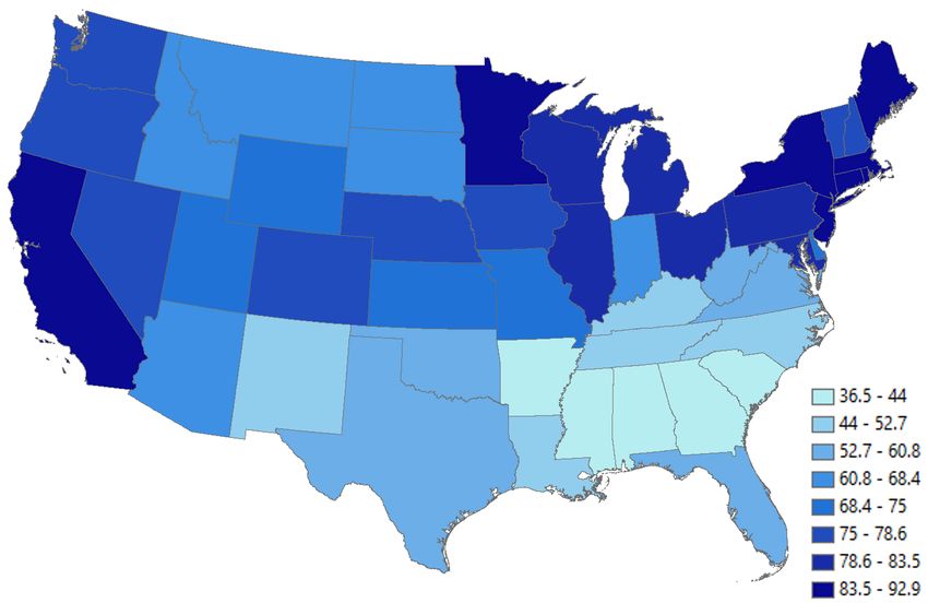
proposed a populist alternative to challenge FDR in the 1936 presidential
election. By the late 1930s, Father Coughlin had become more extreme in his
broadcast and transformed into a major anti-Semitic icon, fascist sympathizer,
and isolationist in pre-war America.
     The episode of Father Coughlin provides a unique opportunity to study
the impact of media manipulation by a charismatic individual. My baseline
analysis examines the impact of exposure to Father Coughlin’s radio program
on voting outcomes in the presidential election of 1936, the year in which
Coughlin harshly attacked the Roosevelt administration. I collect unique data
on the location and technical details of Coughlin’s transmitters in 1936, which
allow me to predict the signal strength of Coughlin’s radio program across
space. Notably, Coughlin’s transmitters changed little over time since 1933,
when he was supporting FDR. It is therefore unlikely that the transmitter
location in 1936 was directly functional to Coughlin’s opposition to FDR.
     Nonetheless, reception of Father Coughlin’s broadcast could be correlated
with other county characteristics that might influence voting outcomes. To
address this concern, I employ a strategy pioneered by Olken (2009) to exploit
the variation in Coughlin’s signal strength resulting from topographic factors.
Specifically, I regress the outcomes on the signal strength of Coughlin’s radio
program, while controlling for the hypothetical signal strength when there is
no geographic or topographic obstacles such as mountains and hills. Hence,
identification comes from the residual variation in signal strength as a result
of idiosyncratic topographic factors along the signal transmission route, which
I find to be uncorrelated with past voting outcomes and a large set of pre-
existing county socioeconomic variables.
     I find that counties more exposed to Father Coughlin’s radio program
displayed lower support for FDR in the 1936 presidential election. Specifically,
a one standard deviation increase in Coughlin signal strength reduced FDR’s
vote share by 2.4 percentage points, or about 4 percent relative to the mean.
The effect was larger in counties with more Roman Catholics, consistent with
Father Coughlin’s greater influence on Catholics.
     To show that the results did not reflect the effect of exposure to radio

                                       3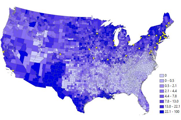
programs in general, I run a falsification test using exposure to national radio
network stations that did not carry Coughlin’s program. In a statistical horse
race between Coughlin and non-Coughlin exposure, I find that what mattered
was exposure to Coughlin’s stations and not exposure to other stations, sug-
gesting that the effect was unique to Coughlin’s radio program.
      Moreover, in another identification strategy, I exploit Coughlin’s switch
in attitude towards FDR during 1932-1936 and panel data during the period
in a difference-in-differences framework. Exploiting within-county variation,
the difference-in-differences strategy controls for any time-invariant differences
across counties and for statewide shocks to counties. Findings from this strat-
egy confirms the baseline results, which also hold under a series of additional
robustness checks, further increasing the causal interpretation of the results.
      Exploring persistence of the effects, I find that exposure to Father Cough-
lin’s broadcast continued to dampen FDR’s vote shares in 1940 and 1944, the
last year in which FDR ran for reelection. The negative effects on Demo-
cratic vote shares became smaller after FDR died in office and persisted in the
following two decades, although declining over time.
      Because of Father Coughlin’s more extreme stance in the late 1930s, I turn
to examine the effects of Coughlin exposure in the late 1930s on anti-Semitism
and civilian support for America’s involvement in WWII. I collect unique data
from FBI records, which allow me to identify all cities with a local branch of
the pro-Nazi German-American Bund in 1940. I find that cities with a one
standard deviation higher exposure to Father Coughlin’s radio program in the
late 1930s were about 9 percentage points more likely to have a local branch
of the pro-Nazi German-American Bund.
      Moreover, using county-level WWII war bond sales data, I find that higher
exposure to Coughlin’s radio program in the late 1930s was also associated with
lower per capita purchase of war bonds. Specifically, a one standard deviation
higher Coughlin exposure was associated with 17 percent lower per capita
purchase of war bonds in 1944, suggesting that Father Coughlin’s isolationist
stance likely dampened public support for the war effort.
      Lastly, using individual survey data from the American National Election

                                        4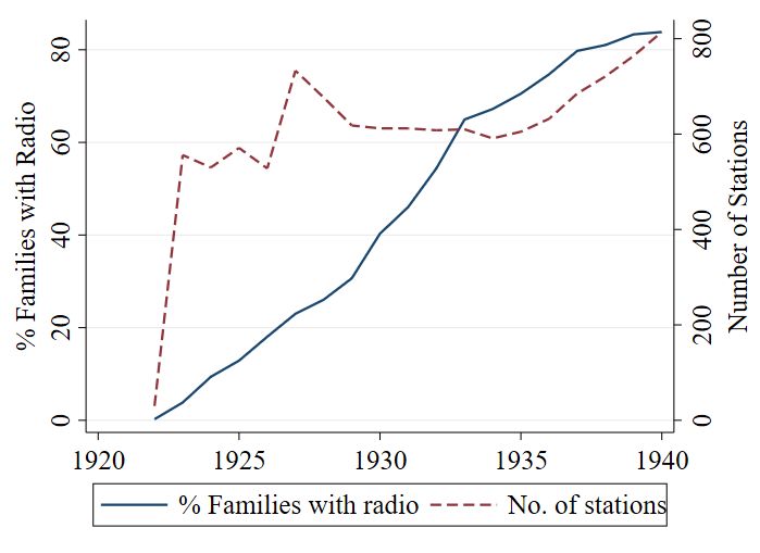
Studies (ANES), I find that individuals in places with a one standard deviation
higher exposure to Coughlin’s broadcast in the late 1930s were associated
with a 1.6 percent rise in negative feelings towards Jews even in the long
run, although the estimate is not precise. In contrast, I do not find such an
association between exposure to Coughlin and feelings towards other minorities
whom Coughlin did not attack, such as blacks or Catholics, suggesting that
the finding does not reflect a change in attitudes towards minorities in general.
      This paper is closely related to the literature on the political persuasion
of media (for surveys of this literature, see DellaVigna and Gentzkow (2010);
Prat and Strömberg (2013); Enikolopov and Petrova (2015); Zhuravskaya et al.
(2019)). Previous work has studied media backed by large institutions, such
as the state or major media organizations.1 This paper focuses on media used
by a charismatic individual, and in particular, a charismatic leader. The po-
litical influence of charismatic individuals, such as politicians, opinion leaders,
and media personalities across a variety of media platforms, has become in-
creasingly evident in recent years, including during the 2016 U.S. presidential
election (Marwick and Lewis, 2017). For instance, the use of Twitter by Don-
ald Trump is widely considered (even by Trump himself) to have contributed to
his election in 2016. Yet, there exists little empirical evidence on the political
impact of media wielded by charismatic individuals.
      I study the extent to which an individual charismatic leader can manip-
ulate the media to influence voting behavior. Related to my work is that of
Garthwaite and Moore (2013) who study the effects of political endorsements
by celebrities. They show that Oprah Winfrey’s endorsement of Barack Obama

   1
     For instance, Adena et al. (2015) finds that radio controlled by Nazi Germany con-
tributed to the support for the Nazi Party and anti-Semitism in Nazi Germany. DellaVigna
and Kaplan (2007) finds that the entry of Fox News increased Republican vote shares in both
U.S. presidential and senatorial elections. Enikolopov et al. (2011) finds that the only inde-
pendent national TV channel in Russia increased votes for opposition parties and reduced
support for the government party in the 1999 parliamentary election. Besides, Durante et al.
(2019) finds that exposure to Italy’s Mediaset all-entertainment TV program increased sup-
port for Berlusconi’s party and for populism in general. An exception, however, is Xiong
(2018), who studies the political premium of TV celebrity and finds that Ronald Reagan’s
tenure as the host of a 1950s entertainment TV program translated into electoral support
during his presidential campaign in 1980.

                                              5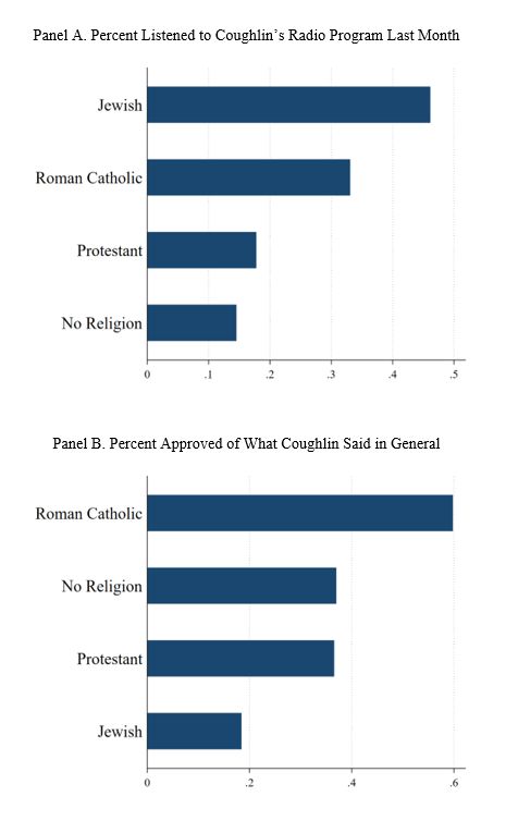
brought approximately 1 million additional votes to him during the 2008 U.S.
Democratic Presidential Primary. In contrast, instead of examining political
endorsements, I focus on the impact of a charismatic demagogue (O’Toole,
2019; Harris, 2009; Warren, 1996; Brinkley, 1982; Bennett, 1969; Lee and Lee,
1939) who uses the media to spread propaganda and misinformation. To my
knowledge, this paper is the first in the literature to empirically document how
a charismatic leader, as an individual, can manipulate the media to influence
voting and political preferences. Moreover, this paper contributes to a broader
literature by exploring the role of religion in political persuasion, which has
gone largely unexplored. Finally, the historical context which I consider pro-
vides a novel opportunity to not only examine short-term effects of exposure
to charismatic leaders, but to also consider the long-term effects of such expo-
sure. While little studied, my results suggest that these long-term effects can
be both statistically and economically significant.
     By exploring arguably the darkest episode of anti-Semitism in American
history, this paper also adds to the literature on media and inter-group an-
imosity (Bursztyn et al., 2019; Müller and Schwarz, 2019a,b; Adena et al.,
2015; DellaVigna et al., 2014; Yanagizawa-Drott, 2014), on religious extrem-
ism (Iannaccone and Berman, 2006), and more specifically, on anti-Semitism
(Becker and Pascali, 2019; Johnson and Koyama, 2019; Finley and Koyama,
2018; Anderson et al., 2017; Voigtlaender and Voth, 2012). Previous work on
anti-Semitism has almost exclusively focused on the European context. Orga-
nized anti-Semitism reached unprecedented levels in inter-war America, and
Father Coughlin is widely considered its foremost proponent (Strong, 1941;
Lee and Lee, 1939). This paper studies an important episode of anti-Semitism
in America, which has received little attention in the literature.
     Furthermore, this paper contributes to the relatively new and growing
literature studying populism. Existing work so far has largely focused on the
determinants of populism, exploring its economic and cultural roots (Ingle-
hart and Norris, 2019; Fukuyama, 2018; Colantone and Stanig, 2018a,b; Autor
et al., 2017; Goodhart, 2017; Gidron and Hall, 2017). There is still little evi-
dence on the extent to which media matter to populist leaders. The findings

                                       6
of this paper are particularly relevant to today’s ongoing debate on the role
of media in the rise of populism (Couttenier et al., 2019; Durante et al., 2019;
Zhuravskaya et al., 2019). Lastly, this paper also contributes to the social
science literature examining Father Coughlin (Warren, 1996; Brinkley, 1982;
Bennett, 1969; Tull, 1965).
2 Historical Background: Radio and Father
Coughlin
Radio as a new communication technology entered American households in
the early 1920s. Providing a variety of music, shows, and information, radio
soon became a popular form of household entertainment. Figure A.1 shows
that the share of American families owning a radio set rose from zero in 1920
to approximately 40 percent by 1930, and it further increased to about 80
percent by 1940; the number of radio stations also increased rapidly during
1920-1940. As a result, the period is often dubbed the Golden Age of Radio.
Radio was central to the rise of Father Coughlin from a local Roman
Catholic priest to a national figure. In 1926, Coughlin started as a priest at
the National Shrine of the Little Flower church in Royal Oak, Michigan, just
outside of Detroit. He quickly embraced radio to broadcast his weekly theolog-
ical teachings from the Detroit station WJR. A charismatic orator on the radio,
Coughlin soon attracted a loyal audience in the Midwest and became known
as the “radio priest.” Indeed, one listener claimed that Coughlin possessed
such a mesmerizing voice “that anyone turning past it almost automatically
returned to hear it again” (Bennett, 1969).
The onset of the Great Depression and the ensuing human suffering, how-
ever, convinced Father Coughlin to switch to broadcast almost exclusively
social and economic commentaries. He described American society as con-
trolled by powerful “banksters,” “plutocrats,” “atheistic Marxists,” and “in-
ternational (commonly understood to mean Jewish) financiers,” whom Cough-
lin blamed for the catastrophe of ordinary American citizens (Warren, 1996).
7Father Coughlin’s outspokenness on the nation’s economic plight brought him
fame as a champion of the common man, but his controversial statements
were often considered demagogic by others (Bennett, 1969; Tull, 1965; Brink-
ley, 1982).
The CBS national network picked up Coughlin’s radio program in 1930,
which made Father Coughlin a household name. Coughlin’s increasingly con-
troversial statements about the economic and financial elites as well as his
refusal to tone down, however, led the CBS to drop his program a year later
(Warren, 1996). In response, Father Coughlin purchased airtime from indi-
vidual stations and formed his own radio network, and his weekly radio show
was soon broadcast again every Sunday afternoon to a national audience. The
Gallup Poll in April 1938 estimated retrospectively that 27.5% of Americans
listened regularly to Father Coughlin’s radio program before the 1936 presi-
dential election.2 This would put Coughlin’s listenership at above 30 million
in the mid-1930s. During the same period, Coughlin also received on aver-
age more than 10,000 unsolicited letters a day from his listeners, often with a
small donation enclosed (Brinkley, 1982). This would make Father Coughlin
the most listened to regular radio speaker as well as the person receiving the
most letters in the world during the 1930s (Brinkley, 1982). It is therefore
not surprising that many contemporary observers regarded Father Coughlin
as the second most influential public figure in the U.S., next only to President
Franklin D. Roosevelt.
Initially a supporter during FDR’s early presidency, Father Coughlin
coined the phrase “Roosevelt or Ruin” in 1933 following FDR’s election (Tull,
1965). Coughlin, however, grew disillusioned with the Roosevelt adminis-
tration over time and deemed the New Deal administration unsuccessful at
addressing the nation’s social and economic problems. In November 1934
Coughlin founded his own organization, the National Union for Social Justice
(NUSJ), to promote ideologies and policies which he believed would lead to
greater prosperity and social justice.3 The Roosevelt administration, however,
2
The number is calculated by the author based on the April 1938 Gallup Poll data from
the Roper Center for Public Opinion Research: https://ropercenter.cornell.edu/
3
Appendix B provides the 16 principles of the National Union Social Justice that Father
8did not follow Coughlin’s proposals. By 1936, Coughlin had become a harsh
denouncer of the Roosevelt administration (Tull, 1965). With the new slogan
“Roosevelt and Ruin,” Father Coughlin accused FDR of being “anti-God”
and a “great betrayer and liar” controlled by both international bankers and
communists.
In 1936, Father Coughlin co-founded a third political party, the Union
Party, together with old-age pension advocate Francis Townsend and Gerald
L. K. Smith, who replaced Huey Long as the head of the Share Our Wealth
movement following Long’s assassination in 1935. The Union Party selected
Republican Senator William Lemke from North Dakota as the party’s candi-
date and proposed a populist alternative to challenge FDR in the 1936 presi-
dential election.
Father Coughlin had become more extreme by the late 1930s. Throughout
1938-1939, Coughlin’s radio broadcast and weekly newspaper, Social Justice,
were overtly anti-Semitic (Warren, 1996). He portrayed Jews as malicious
aliens associated with communism and made bitter personal attacks on lead-
ing rabbis and Jewish organizations (O’Toole, 2019). He blamed Jews for
inciting the European conflicts, supported pro-Nazi organizations in America
such as the German-American Bund, and serialized in his weekly newspaper
the Protocols of the Elders of Zion, the notorious fake document purporting
Jewish plans for world domination (O’Toole, 2019). Some of Father Coughlin’s
writings in his newspaper even followed Joseph Goebbels’ speeches verbatim
(Warren, 1996). In 1938, Coughlin also played an instrumental role in form-
ing a paramilitary and anti-Semitic organization, the Christian Front, which
specialized in harassing and beating up Jews and vandalizing Jewish prop-
erty across major U.S. cities (O’Toole, 2019). Besides, Father Coughlin was
also a staunch supporter for American isolationism. Calling FDR “the world’s
chief warmonger,” Coughlin vehemently opposed America’s entry into WWII
and endorsed the leading U.S. isolationist organization, the American First
Committee.
Father Coughlin’s controversial activities eventually led to his downfall.
Coughlin outlined at its founding in November 1934.
9In late 1939, the National Association of Broadcasters (NAB) introduced a
new self-regulation code that prohibited radio stations from discussing contro-
versial issues in sponsored programs, a rule that many believe was introduced
specifically to rein in Father Coughlin (Warren, 1996). Following this new rule,
almost no station were willing to sell Coughlin airtime, which forced him off the
air in 1940. Shortly following the Pearl Harbor attack, the federal government
further invoked the Espionage Act of 1917 and banned postal circulation of
Coughlin’s weekly newspaper in 1942 because of its seditious content. Church
superiors also ordered Coughlin to relinquish any political involvement or to
give up his priesthood. Father Coughlin chose to return to his parish duties
in 1942 and refrained from the public sphere thereafter.
3 Data
My baseline empirical work relates exposure to Father Coughlin’s anti-FDR
broadcast in 1936 to voting outcomes in the 1936 presidential election. In
this section, I describe the data employed in the baseline analysis, including
data used to measure exposure to Father Coughlin’s radio program, electoral
outcomes, and other county characteristics.
3.1 Exposure to Father Coughlin’s Radio Program
A challenge to study Father Coughlin’s impact on the 1936 presidential elec-
tion is the lack of data measuring exposure to Coughlin’s radio program in
1936 at a fine-grained geographic level. For this project, I assemble a unique
data set from several sources that is particularly suited to measure the political
impacts of Father Coughlin. To proceed, I identify all the radio stations that
Coughlin used for his weekly broadcasts in 1936 from the historical magazine
Broadcasting. Figure A.2 displays the location of the stations, showing a total
of 33 stations. For each of Coughlin’s station, I collect technical details from
the 1936 Broadcasting Yearbook, which provide me with the transmitter fre-
quency, power, and height. I then use this information to calculate the signal
10strength of Father Coughlin’s radio program across U.S. counties in 1936.
Radio signal transmission obeys the laws of electromagnetic propagation.
In the free space (i.e. assuming the earth is smooth and without any geo-
graphic or topographic obstacles), signal strength is inversely proportional to
the square of the distance from the transmitter (Olken, 2009). In actual trans-
mission, however, the presence of geographic or topographic obstacles, such as
mountains or hills, would lead to diffraction and greater transmission loss in
signal. I calculate the signal transmission loss with a professional radio prop-
agation software based on the Irregular Terrain Model (ITM). The ITM was
developed by the U.S. government in the 1960s and typically used by radio
and TV engineers to predict signal strength of broadcasts.4
Following Olken (2009), I calculate the transmission loss for each transmitter-
county pair using the ITM algorithm.5 I then deduct the transmission loss from
the power of the transmitter to get the predicted signal strength, where signal
strength is measured in decibel-milliwatts (dBm). Finally, for each county
I use the maximum predicted signal strength across all transmitters as the
predicted signal strength in that county.
Panel A of Figure 1 shows the predicted signal strength of Father Cough-
lin’s radio program across counties, where stronger signals are shown with
darker colors.6 Previous studies (Olken, 2009; Enikolopov et al., 2011; Adena
et al., 2015) have shown that signal strength is a strong predictor for the actual
audience size. Because county-level listenership data of Coughlin’s radio pro-
gram are not available, I follow Durante et al. (2019) and use the continuous
4
Benjamin Olken has kindly shared the software with me. The ITM software has also
been used to calculate radio signal strength in historical settings by Adena et al. (2015)
in the context of Nazi Germany and by Gagliarducci et al. (ming) in the context of Italy
during WWII.
5
I use the centroid of each county as the receiving location.
6
Evidently the Cincinnati station is the most powerful station, with its signal dominating
a large number of counties. This is because the Cincinnati station WLW was chosen by the
federal government to experiment with high power broadcasting and authorized to broadcast
at 500 kW between 1935 and 1939, while all other stations were operating at 50 kW or less.
WLW was one of Coughlin’s stations in 1936. My results are robust to simply removing this
station from Coughlin’s radio network or using 50 kW as its power, which was its original
power before 1935, to calculate the signal strength. Hence, my results are not driven by the
Cincinnati station.
11measure of signal strength as the explanatory variable.7 Nonetheless, Figure
A.5 provides evidence that the share of population who regularly listened to
Coughlin before the 1936 election was highly correlated with the location of
his stations and with the predicted signal strength across regions.
It is also evident from Figure A.2 that Father Coughlin had no station
in the geographic South. This has been attributed to the fact that Coughlin
would have attracted few audience in the South as a Catholic priest of Irish
descent (Tull, 1965). Indeed, Figure A.3 maps the spatial distribution of the
Catholic population in 1926 and shows that the location of Father Coughlin’s
stations largely followed the the pre-existing spatial distribution of Catholics,
which the South had few. In addition, the South also had a relatively lower
radio ownership than the rest of the nation, as seen in Figure A.4.
Because the South had much fewer potential listeners of Father Coughlin
regardless of Coughlin’s signal strength in the region, I focus my empirical
analysis on states outside of the geographic South to improve precision.8 The
central results are qualitatively similar when I include all states in my analysis.
I use the ITM to also generate the hypothetical signal strength in the
free space, assuming the earth is free of any geographic or topographic obsta-
cles that may hinder signal transmission. This is important to my baseline
identification strategy which exploits the varying topography along the signal
transmission route to provide plausibly exogenous variation in signal strength,
a point I will return to in Section 4.
7
The Gallup Poll in April 1938 asked retrospectively about Coughlin listenership before
the 1936 election. The data unfortunately do not contain county identifiers for individual
respondents. While I use the continuous measure of signal strength in most of my analysis,
in a robustness check I use an indicator variable that equals 1 if a county’s signal strength
is above median and 0 otherwise.
8
Indeed, Figure A.5 shows that the South had the lowest Coughlin listenership among
all regions before 1936 election. The 11 Southern states excluded are Oklahoma, Arkansas,
Tennessee, North Carolina, Texas, Louisiana, Mississippi, Alabama, Georgia, Florida, and
South Carolina. Including these states produces qualitatively similar results for my baseline
estimates, which I will show in Table A.2 as a robustness check.
123.2 Voting Data and County Characteristics
The main outcomes of interest of my baseline analysis consist of vote shares
(in percentage points) of the Democratic Party (FDR), the Republican Party,
and other parties in each county in the 1936 presidential election. Some of my
analyses also use vote shares from past and later presidential elections. These
data come from the ICPSR Study 8611 data set (Clubb et al., 2006). Figure
A.6 shows FDR’s vote share across counties in the 1936 presidential election.
County-level socioeconomic variables are obtained from several sources.
From the ICPSR 2896 data set (Haines, 2010), I obtain a rich set of 1930
county demographics, measuring county population and population by gen-
der, race, birth place, age, literacy, employment status, radio ownership, and
farm characteristics. I use the 1930 Census IPUMS microdata to compute for
each county its mean occupational income score and shares of employment
in manufacturing and in agriculture. The 1926 Census of Religious Bodies
provides me with the share of population belonging to each religious denomi-
nation at the county level in 1926, which allows me to measure the population
share of Roman Catholics. I use ArcGIS to generate additional county-level
geographic characteristics, including area, elevation, and terrain ruggedness.9
4 Empirical Strategy
The objective of my baseline empirical work is to study the impact of exposure
to Father Coughlin’s radio program on voting outcomes in the 1936 presidential
election. Notably, the location of Father Coughlin’s stations in 1936 were
mostly the same as that in 1933, when Coughlin was supportive of FDR.
Figure A.2 maps Coughlin’s stations in 1936, which shows that 25 out of the
33 (or about 76%) stations in 1936 were already in Coughlin’s network in 1933,
when Coughlin was still a strong supporter for FDR. It is therefore unlikely
that station location in 1936 was intentionally driven by Coughlin’s opposition
9
I measure elevation and ruggedness at county centroids, consistent with what I did for
signal strength.
13to FDR.10
Nonetheless, reception of Coughlin’s broadcast might have been corre-
lated with other local characteristics (e.g. distance to major cities) that could
have influenced voting behavior in 1936. To address this concern, I employ an
empirical strategy pioneered by Olken (2009) and exploit plausibly exogenous
variation in Coughlin’s signal strength resulting from topographic factors.11
Specifically, I regress the outcomes of interest on the actual signal strength
(Signal), while controlling for the hypothetical signal strength in the free
space (SignalF ree) where the earth is assumed to be free of any topographic
obstacles, such as mountains or hills, that diffract and weaken radio signal
transmission. Crucially, the variable SignalF ree controls for a county’s prox-
imity to a transmitter as well as the power of the transmitter. Therefore, once
controlling for SignalF ree, identification of the coefficient of Signal comes
from variation in diffraction patterns caused by topographic obstacles along
the signal transmission route. Figure 1 shows the actual (ITM-predicted) sig-
nal strength of Coughlin’s radio program and the hypothetical signal strength
in the free space.
Because a county’s own topography could also potentially influence its
political outcomes, I control for various local geographic characteristics of the
county, including the county’s surface area, altitude, and terrain ruggedness
as well as the square terms of each of these geographic variables. Therefore, I
only exploit residual variation in signal strength resulting from the topography
along the signal transmission route outside the county, which is arguably more
exogenous.12 Furthermore, I include state fixed effects to compare counties
within the same state in all my analyses.
I run the following regression for my baseline analysis:
10
While Coughlin’s radio network clearly expanded westward between 1933 and 1936,
the results are robust to restricting the sample to counties only in the Northeast and the
Midwest, where station location changed little over time.
11
A similar strategy has also been used by Durante et al. (2019), DellaVigna et al. (2014),
and Yanagizawa-Drott (2014).
12
The exceptions are the counties that contained Coughlin stations. I will provide ro-
bustness checks by dropping these counties as well as the areas surrounding them.
14V otec = βSignalc + γSignalF reec + δ 0 Xc + ηs + c (1)
where V otec is the vote share (in percentage points) received by a party in
county c in the 1936 presidential election. Signalc is the actual signal strength
of Father Coughlin’s radio program in county c in 1936. SignalF reec is the
hypothetical signal strength in the free space. Xc is a vector of county baseline
controls for local geographic characteristics, socioeconomic characteristics, and
past voting outcomes. ηs are state fixed effects, controlling for any differences
across states that might influence voting. c is the error term. Standard errors
are corrected for clustering at the state level. To ease the interpretation of
the results, I standardize signal strength such that it has a mean of zero and
a standard deviation of one.
The coefficient β provides the reduced-form estimate of the effect of ex-
posure to Father Coughlin’s radio program. The identification assumption
is that Signal is not correlated with unobserved factors that influence voting
outcomes, conditional on all the covariates in equation (1). While the assump-
tion is ultimately untestable, I support the conditional exogeneity assumption
through balance and placebo tests by examining the correlation of Signal with
pre-existing county socioeconomic characteristics and past voting outcomes.
In Table 1, I examine the correlation between Coughlin’s signal strength
in 1936 and 1930 county socioeconomic characteristics. As seen in column 2,
Signal is significantly correlated with quite a few socioeconomic variables in
the univariate regression. This is not surprising given that Father Coughlin’s
stations were mostly in large cities in the Northeast and the Midwest. Signal,
however, becomes more balanced across the set of 17 socioeconomic character-
istics after I control in column 4 for the free-space signal, state fixed effects,
and local geographic characteristics. In fact, SignalF ree, state fixed effects,
and local geographic characteristics explain about 30-60 percent of the overall
variation of most of the socioeconomic variables. Conditional on the additional
covariates, Signal is no longer correlated with most pre-existing demographic
or industrial characteristics, although it is still correlated with the share of el-
derly, unemployment rate, and radio ownership. To be conservative, I include
15all the socioeconomic characteristics in Table 1 as controls in equation (1).
In Table 2, I perform a series of placebo tests by examining the correlation
between Signal and Democratic and Republican vote shares in past presiden-
tial elections before 1936. Conditional the full set of baseline controls, Signal
is not significantly correlated with any of the past electoral outcomes dur-
ing the period 1920-1932 (column 1-8) or with changes in electoral outcomes
between 1928 and 1932 (column 9-10); the estimated coefficients are also gen-
erally small. The results suggest that exposure to Father Coughlin’s radio
program in 1936 was not systematically correlated with pre-existing politi-
cal preferences in either levels or trends, providing support to the conditional
exogeneity assumption of equation (1).
5 Father Coughlin and Presidential Elections
In this section, I present the results on the impact of exposure to Father
Coughlin’s radio program on presidential election voting outcomes. I focus on
the presidential election of 1936, the year in which Father Coughlin harshly
attacked FDR in his radio broadcasts and co-founded the Union Party to
challenge FDR in the presidential race.
5.1 Baseline Results
Table 3 shows the estimated effects of exposure to Father Coughlin’s broad-
cast on voting in the 1936 presidential election. I find that exposure to Father
Coughlin’s radio program had a large negative effect on the support for FDR in
the 1936 presidential election. Based on column 1, without any control, a one
standard deviation increase in exposure to Father Coughlin’s radio program
was associated with a reduction in FDR’s vote share by about 3.8 percentage
points. The results are robust and of similar magnitudes when adding in differ-
ent controls in subsequent columns, including state fixed effects, the free-space
signal, and county geographic and socioeconomic characteristics. In column 6,
after further controlling for past electoral outcomes, the estimated coefficient
16changes little. Based on column 6, which is my preferred specification that
includes all baseline controls, a one standard deviation increase in exposure to
Coughlin’s radio program reduced FDR’s vote share by about 2.4 percentage
points, which is about 4 percent relative to the mean of FDR’s vote share.
Column 7 of the table, which uses the Republican Party’s vote share as the
outcome, shows that most of the reduction in FDR’s vote share as a result of
exposure to Coughlin went to the Republican Party. A one standard deviation
increase in exposure to Coughlin’s radio program increased the Rupublican
vote share by about 2 percentage points. The voting data set unfortunately
does not contain separate voting results for different third parties in 1936, even
though the Union Party received most of the votes among third parties.13
The data limitation makes it difficult to examine the effect on the Union
Party specifically. I therefore combine the vote shares of all other parties into
one category and use it as the outcome in Column 8. Column 8 shows that
exposure to Father Coughlin increased the support for other parties by about
0.4 percentage points, although the effect is not precisely estimated. Taken as
a whole, Table 3 suggests that exposure to Father Coughlin’s radio program
reduced support for FDR in the 1936 presidential election.
Next, I turn to examine the role of religion in Father Coughlin’s persua-
sion. As a Roman Catholic priest, Father Coughlin likely had greater influence
among the Catholic population. Indeed, based on a Gallup Poll survey in De-
cember 1938, Panel B of Figure A.7 shows that more than 60% of Catholics
approved of what Father Coughlin said in general, much higher than other re-
ligious groups did. I therefore expect that exposure to Father Coughlin’s radio
program to have a larger effect in counties with more Catholics. To test this
hypothesis, I include in my regression interaction terms between Signal and an
indicator variable that equals 1 if a county’s population share of Catholics was
in the top quartile of the distribution among all counties and 0 otherwise.14
Table 4 reports the estimates based on this regression. Consistent with
13
In 1936, votes for the Union Party represented 73.5% of all the votes that went to third
parties.
14
Results based on a continuous measure of the population share of Catholics are similar
and shown in Table A.1.
17the expectation, the effects estimated are larger in highly Catholic counties.
Here the effect of Signal in highly Catholic counties is equal to the sum of
the coefficient on Signal and that on the interaction term Signal × Catholic.
Based on column 1, a one standard deviation increase in Coughlin exposure
reduced FDR’s votes by about 3.4 percentage points in highly Catholic coun-
ties. Column 2 shows that there was no differential effect on the support for
the Republican Party in highly Catholic counties. In contrast, Coulumn 3
shows that a one standard deviation increase in Coughlin exposure increased
the support for other parties by about 1.4 percentage points in highly Catholic
counties, which most likely reflect an increase in support for Coughlin’s Union
Party since it was the dominant third party in 1936. Taken together, Table 4 is
consistent with Father Coughlin having a greater influence on Catholic voters
and suggests the possibility for religion to be exploited for political persuasion.
A potential concern remains that the baseline results may simply reflect
exposure to radio programs in general instead of exposure to Father Cough-
lin. To address this concern, I collect data on NBC and CBS network radio
stations that did not carry Coughlin’s broadcast and run a falsification test.
Specifically, I use the same method to predict the signal strengths from the
non-Coughlin stations and then include the non-Coughlin signal strengths (in-
cluding free-space signals) in my baseline regression to perform a statistical
horse race. Table 5 reports these results. As seen in Table 5, the estimated
effects of exposure to non-Coughlin stations are much smaller in magnitude
and statistically insignificant, while the estimates for exposure to Coughlin’s
stations remain strong and similar as in the baseline. The statistical horse race
between Coughlin and non-Coughlin stations suggests that it was exposure to
Father Coughlin’s radio program, instead of exposure to radio programs in
general, that reduced support for FDR in 1936.
5.2 Evidence from a Difference-in-Differences Strategy
A unique feature of my empirical setting is Father Coughlin’s switch in his
attitude towards FDR between 1932 and 1936. Although Father Coughlin
18was pro-FDR in the 1932 presidential election, Coughlin did not explicitly
broadcast his support for FDR in his radio program until FDR had won the
election (Warren, 1996; Tull, 1965). In a private letter written to FDR during
the 1932 presidential campaign, Father Coughlin expressed strong support for
FDR but stated that he could not take a stand publicly or endorse a particular
candidate because his priesthood forbade him to do so (Tull, 1965). Yet, by
1936, Coughlin had taken an explicit stand against FDR and made that public
through his radio program. Therefore, I would expect places more exposed to
Father Coughlin’s radio program in 1936 to display a greater reduction in
support for FDR between 1932 and 1936.
To exploit the change in Father Coughlin’s attitude between 1932 and
1936, I turn to a difference-in-differences specification using the 1932-1936
panel and exploit only within-county variation over time. Specifically, I run
the following regression:
V otect = βSignalc × P ostt + Xc × P ostt + σc + ηst + ct (2)
where Signalc is the predicted signal strength of Father Coughlin’s radio pro-
gram in county c in 1936. P ostt is an indicator for post-1932, which equals
1 in 1936 and 0 in 1932. σc are county fixed effects, which control for any
time-invariant county characteristics. ηst are state-by-year fixed effects, which
control for statewide shocks to all counties in each state. In some specifica-
tions, I further control for the interactions between all my baseline county
characteristics Xc and P ostt , which allow each baseline county characteris-
tic to have a differential effect on voting over time. The standard errors are
corrected for clustering at the county level.
Table 6 reports the results from the difference-in-differences specification,
which substantially confirm the baseline results. Column 1 of Table 6 shows
that, controlling for county fixed effects and year fixed effects, a one standard
deviation increase in exposure to Father Coughlin’s radio program decreased
FDR’s vote share by about 1.5 percentage points. The estimated effects re-
main robust after controlling for state-by-year fixed effects in column 2 and, if
anything, become slightly larger when controlling for the interactions between
19baseline county characteristics and the P ost dummy in column 3. Column 4
and 5 of the table show that the estimated effects for the Republican party
and for other parties remain similar in magnitudes as found in the baseline
and become more precisely estimated.
The identifying assumption of the difference-in-differences specification is
that vote shares in counties with different levels of exposure to Father Coughlin
would have followed parallel trends absent of Father Coughlin’s radio program.
Results in columns 9 and 10 of Table 2 are consistent with the parallel trends
assumption by showing that exposure to Coughlin’s radio program in 1936
was not significantly correlated with changes in vote shares during 1928-1932.
Here, I provide additional support for the parallel trends assumption using an
event study on a relatively longer panel. Specifically, I run equation (2) on
the panel of 1912-1944, replacing P ostt with year dummies and using 1932
as the omitted category. The period of 1912-1944 covers all four presidential
elections (1932-1944) involving FDR as well as five elections before.
Figure 2 presents the event study graph for Democratic vote shares. As
seen from this figure, the estimates in the five pre-periods are relatively small in
magnitudes and not significantly different from that in 1932; the lack of a clear
trend before 1936 supports the parallel trends assumption. The estimates for
the period 1936-1944 suggest that higher exposure to Father Coughlin’s radio
program in 1936 reduced support for FDR in each of FDR’s re-elections since
1936. The negative effects appear to increase in magnitude over time. Based
on the 1944 estimate, relative to FDR’s vote share in 1932, a one standard
deviation higher exposure to Father Coughlin’s radio program lowered FDR’s
vote share by about 3.7 percentage points in the 1944 election. Overall, the
event study exercise largely confirms the baseline findings.
5.3 Additional Robustness Checks
I perform several additional robustness checks on my baseline results using
FDR’s 1936 vote share as the outcome variable and report them in Table A.2.
In column 1 of the table, I verify that the results are not driven by particular
20parametric assumptions by using a binary measure of signal that equals 1 if
the signal strength was above the median and 0 otherwise. The results are
robust to using the binary measure. In column 2, I drop counties within 100
miles from any Coughlin’s stations in 1936 to verify that big cities or their
surrounding regions do not drive the results.15 Counties further away from a
station generally had a smaller population and their exposure to Coughlin’s
broadcast was more likely exogeneous.
In column 3, I control for the free-space signal more flexibly, including the
squared and the cubic terms of the the free-space signal in the baseline regres-
sion as additional controls. The results still hold. Column 4 shows that the
results are also robust to controlling for county-level New Deal expenditures
using data from Fishback et al. (2003), including per capita New Deal grant,
relief, and loans.
In column 5, I examine the effect on the full sample of counties including
the South. The coefficient becomes somewhat smaller and less precisely esti-
mated (p-value = 0.104), possibly because of Father Coughlin’s much lower
listenership in the South. But the result is qualitatively similar and indicates
an overall negative effect of exposure to Father Coughlin on voting for FDR in
1936. In column 6, I weight the baseline regression using county population,
and the estimate changes little. The robustness of the results to this series of
additional checks further support the causal interpretation of the results.
5.4 Persistence after 1936
Father Coughlin was forced off the air in the spring of 1940. Did exposure to
Father Coughlin’s radio program have persistent effects on presidential voting
in the long run? To explore this question, I turn to examine the effects of
exposure to Father Coughlin in 1936 on voting outcomes in later presidential
elections.
While Figure 2 shows that exposure to Father Coughlin continued to
negatively affect FDR when FDR ran for re-elections in 1940 and 1944, it is
15
The results are qualitatively similar when focusing on counties that were 150, 200, 250
or 300 miles away from any Coughlin’s stations.
21less clear how early exposure to Father Coughlin would affect later presidential
voting after FDR passed away in office in 1945, five years after Coughlin left
the air. The negative effects on the Democratic Party could vanish after 1945
if voters associated Coughlin’s attacks only with FDR himself, and the effects
could persist if voters associated the attacks on the New Deal and the Roosevelt
administration with the Democratic party.
Figure A.8 plots the estimated coefficients on Signal from separate re-
gressions, in which the outcomes are the Democratic vote shares in each pres-
idential election from 1936 and 1972, the last year covered by the ICPSR
Study 8611 dataset (Clubb et al., 2006). The figure shows that exposure to
Father Coughlin continued to negatively affect the Democratic vote shares in
the long run. The effects, however, appear to decrease after FDR passed away
in 1945 and decline over time until disappearing in 1972. The persistence of
the effects suggests that Father Coughlin’s attack on the Roosevelt adminis-
tration possibly shaped many voters’ attitudes towards the Democratic party
and highlights the impact of influential opinion leaders like Father Coughlin.
6 Father Coughlin, Anti-Semitism, and Civil-
ian Support for WWII
By the late 1930s, Father Coughlin had become a leading anti-Semitic icon,
fascist sympathizer, and isolationist advocate in pre-war America (Tull, 1965;
Brinkley, 1982; Warren, 1996). I now turn to examine the impact of Coughlin’s
radio broadcast on measures of anti-Semitism, fascist sympathies, and support
for the war effort among Americans.
6.1 Civilian Support for America’s War Effort
First, I examine whether exposure to Father Coughlin’s radio program affected
civilian support for America’s war effort during WWII. To carry out this ex-
ercise, I use data on county-level WWII bond sales in 1944, which come from
the 1947 County and City Yearbooks. I divide total bond sales by county pop-
22ulation to obtain per capita sales of WWII bonds in each county. For the ease
of interpretation, I use the natural log of per capita war bond sales as the
outcome variable. To measure exposure to Father Coughlin’s radio program,
I collect data on Coughlin’s stations in 1939 and use the ITM software to
measure their signal strength across counties as I did in the baseline analysis.
I then run a similar regression as in equation (1), regressing war bond sales in
1944 on the signal strength of Coughlin’s radio program in 1939.
Table 7 reports the results from this exercise. To be consistent with my
baseline results, I again focus on regions outside of the geographic South.16
Across different specifications, exposure to Father Coughlin’s radio program
in 1939 is associated with lower per capita war bond sales in 1944. Based on
column 5, conditional on all the controls, a one standard deviation increase in
Coughlin signal is associated with a 17% decrease in per capita WWII bond
sales. The results suggests that exposure to Father Coughlin’s radio program
in the late 1930s lowered civilian support for America’s war effort.
6.2 Evidence from the German-American Bund
In a broadcast following Nazi Germany’s Kristallnacht in November 1938,
Father Coughlin notoriously labeled the attacks on Jews as a defense against
communism (Warren, 1996). Based on the December 1938 Gallap Poll, Figure
A.7 shows that while close to 60% of Catholics approved of what Coughlin
said in general, less than 20% of Jews did. It is natural to wonder whether
exposure to Father Coughlin’s anti-Semitic broadcasts throughout the period
of 1938-1939 affected anti-Semitism in America.
A challenge to study anti-Semitism or fascist sympathies in pre-war Amer-
ica, however, is the lack of data measuring these outcomes. To overcome the
challenge, I collect new data from the FBI records on the German-American
Bund, the leading anti-Semitic and pro-Nazi organization in pre-war America
(Strong, 1941). The data allow me to identify all the cities with a local branch
of the Bund in 1940, a total of 54 cities.
16
Results based on the full sample of counties are qualitatively similar and remain sta-
tistically significant at the 5 percent level.
23I conduct a similar exercise as in the baseline analysis at the city level.
I define the outcome to be a binary variable that equals 1 if a city had a
local branch of the Bund in 1940, and 0 otherwise. The explanatory variable
is city-level signal strength of Coughlin’s radio program in 1939. Since the
smallest city with a local branch of the Bund had a population of 11,710, I
define the sample to consist of all identifiable cities in the 1930 Census that
had a population of 10,000 or above. I then regress whether the city had a
branch of the Bund on Coughlin’s signal strength in 1939, controlling for the
free space signal, city characteristics, and state fixed effects.
Table 8 reports the results from this exercise. In column 1, I control for
only the free space signal and state fixed effects. In column 2, I add controls
for city geographic characteristics, including elevation and its square, as well
as terrain ruggedness and its square. In column 3, I further control for city
socioeconomic characteristics as observed in 1930, including population, per-
cent unemployed, average occupational income score, percent owning a radio,
perccent of Jewish descent, percent of first- or second-generation German im-
migrants, percent native, and an indicator for large city (having a population
above 100,000).17 Based on column 3, a one standard deviation increase in
Coughlin exposure was associated with about a 9 percentage points higher
likelihood of having a local branch of the German American Bund. In column
4, I restrict my sample to only those cities more than 50 miles away from
a Coughlin station, whose exposure to Coughlin’s radio program was more
likely to be exogenous, and the estimate changes little. Overall, Table 8 offers
suggestive evidence that Father Coughlin’s radio program possibly increased
fascist sympathies and anti-Semitic sentiment in pre-war America.
17
I measure population of Jewish descent by counting individuals whose mother tongues
were either Yiddish or Hebrew in the 1930 Census. I measure population of first- or second-
generation German immigrants by counting individuals whose mother tongues were German
or who had at least one parent born in Germany in the 1930 Census.
246.3 Public Attitudes towards Jews in the Long Run
Lastly, to explore the impact of Father Coughlin’s radio program on the public
attitudes towards Jews in the long run, I turn to individual survey data from
the nationally representative American National Election Studies (ANES).
Since the 1960s, the ANES have asked about respondents’ feelings towards
Jews in several rounds of surveys using a feeling thermometer question.18
Specifically, the question asked about the respondents’ feelings of warmth to-
wards Jews (and other groups of people) on a scale from 0 to 100, with 100
being the warmest. I use this feeling thermometer variable (ranging from 0
to 100) as the outcome and run a similar regression as in equation (1) at the
individual level. To do that, I pool together all ANES surveys in which feeling
thermometer measurements on Jews are available, including the years of 1964,
1966, 1968, 1972, 1976, 1988 and 1992. This provides me with more than
11,500 individuals from 228 counties. I measure exposure to Coughlin’s anti-
Semitic radio program using the predicted signal strength of Coughlin’s radio
program across counties in 1939. The county identifiers in the ANES data
allow me to assign exposure to Father Coughlin’s radio program to individuals
based on the counties they lived in. Unfortunately, the ANES survey did not
ask about the counties in which the respondents grew up, which would more
likely capture exposure to Coughlin. Therefore, the results from this exercise
should be interpreted with more caution.
Table 9 reports the results from this exercise. Columns 1 to 6 of the table
show that individuals living in places more exposed to Father Coughlin’s radio
program in 1939 displayed more negative feelings towards Jews in the long
run. Based on the estimates, in general a one standard deviation increase in
Coughlin exposure is associated with an approximately 1 percentage point drop
(out of a mean of 63 percentage points) in positive feelings towards Jews, or
about a 1.6 percent decrease. The estimate becomes statistically insignificant
in column 6 after controlling for state fixed effects, although the magnitude
remains sizable and negative.
18
The data come from the ANES Time Series Cumulative Data File (1948-2012) (ICPSR
8475).
25You can also read