MHD study of planetary magnetospheric response during extreme solar wind conditions: Earth and exoplanet magnetospheres applications
←
→
Page content transcription
If your browser does not render page correctly, please read the page content below

Astronomy & Astrophysics manuscript no. Earth_CME__referee                                     ©ESO 2022
                                              March 7, 2022

                                              MHD study of planetary magnetospheric response

                                              during extreme solar wind conditions: Earth and

                                                        exoplanet magnetospheres applications

                                                  J. Varela1 , A. S. Brun2 , A. Strugarek2 , V. Réville3 , P. Zarka4 , and F. Pantellini5
arXiv:2203.02324v1 [astro-ph.EP] 4 Mar 2022

                                                  1
                                                      Universidad Carlos III de Madrid, Leganes, 28911
                                                      e-mail: jvrodrig@fis.uc3m.es
                                                  2
                                                      Laboratoire AIM, CEA/DRF – CNRS – Univ. Paris Diderot – IRFU/DAp, Paris-Saclay, 91191
                                                      Gif-sur-Yvette Cedex, France
                                                  3
                                                      IRAP, Université Toulouse III—Paul Sabatier, CNRS, CNES, Toulouse, France
                                                  4
                                                      LESIA & USN, Observatoire de Paris, CNRS, PSL/SU/UPMC/UPD/UO, Place J. Janssen,
                                                      92195 Meudon, France
                                                  5
                                                      LESIA, Observatoire de Paris, Université PSL, CNRS, Sorbonne Université, Université de
                                                      Paris, 5 place Jules Janssen, 92195 Meudon, France

                                                  version of March 7, 2022

                                                                                             ABSTRACT

                                                  Context: The stellar wind and the interplanetary magnetic field modify the topology of planetary
                                                  magnetospheres. Consequently, the hazardous effect of the direct exposition to the stellar wind,
                                                  for example regarding the integrity of satellites orbiting the Earth or the habitability of exoplan-
                                                  ets, depend upon the space weather conditions.
                                                  Aims: The aim of the study is to analyze the response of an Earth-like magnetosphere for various
                                                  space weather conditions and interplanetary coronal mass ejections. The magnetopause stand off
                                                  distance, open-close field line boundary and plasma flows towards the planet surface are calcu-
                                                  lated.
                                                  Methods: We use the MHD code PLUTO in spherical coordinates to perform a parametric study
                                                  regarding the dynamic pressure and temperature of the stellar wind as well as the interplanetary
                                                  magnetic field intensity and orientation. The range of the parameters analyzed extends from reg-
                                                  ular to extreme space weather conditions consistent with coronal mass ejections at the Earth orbit
                                                  for the present and early periods of the Sun´s main sequence. In addition, implications of sub-
                                                  Afvenic solar wind configurations for the Earth and exoplanet magnetospheres are analyzed..
                                                  Results: The direct precipitation of the solar wind at the Earth day side in equatorial latitudes is

                                                                                                                              Article number, page 1 of 63
Varela et al.: Planetary magnetospheric response during extreme solar wind conditions

      extremely unlikely even during super coronal mass ejections. On the other hand, for early evo-
      lution phases along the Sun main sequence once the Sun rotation rate was at least 5 times faster
      (< 440 Myr), the Earth surface was directly exposed to the solar wind during coronal mass ejec-
      tions. Nowadays, satellites at High, Geosynchronous and Medium orbits are directly exposed to
      the solar wind during coronal mass ejections, because part of the orbit at the Earth day side is
      beyond the nose of the bow shock.

      Key words. Earth magnetosphere – space weather – CME – Earth habitability

1. Introduction

The space weather forecasting in the last decades has shown the important effect of the solar wind
(SW) and interplanetary magnetic field (IMF) on the Earth magnetosphere, ionosphere, thermo-
sphere and exosphere state (Poppe, B.B. & Jorden, K.P. 2006; González Hernández, I. et al. 2014).
Physical phenomena as geomagnetic storms (Gonzalez, W. D. et al. 1994) and substorms (Baker,
D. N. et al. 1999), energization of the Van Allen radiation belts (Shah, A. et al. 2016), ionospheric
disturbances (Cherniak, I. & Zakharenkova, I. 2018), aurora (Zhang, Y. & Paxton, L. J. 2016), and
geomagnetically induced currents at Earth’s surface (Pulkkinen, A. et al. 2017) are triggered dur-
ing particular space weather conditions. Extreme space weather conditions linked to coronary mass
ejections (CME) lead to a strong perturbation of the Earth magnetosphere (Cane, H. V. et al. 2000;
Richardson, I. G. et al. 2001; Wang, Y. M. et al. 2003; Lugaz, N. et al. 2015; Wu, C. & Lepping, R.
P. 2015). The list of consequences is large: failure of spacecraft electronics due to radiation damage
and charging (Choi, H.-S. et al. 2011), enhancement of the drag on low orbit satellites (Nwankwo,
V.U.J. et al. 2015), spacecraft signal scintillation due to a perturbed ionosphere (Molera Calvés,
G. et al. 2014), ground induced electric currents that can cause the collapse of electric power grids
(Cannon, P. et al. 2013), ionizing radiation that harms astronauts and passenger of the commercial
aviation (Bazilevskaya, G.A. 2005), among others. Recently, the analysis of the space weather is
generalized for the case of stars different than the Sun (Strugarek et al. 2015; Garraffo, C. et al.
2016). Between other factors, the habitability of the exoplanets depends on the space weather con-
ditions imposed by the hosting star and the shielding efficiency of the exoplanet magnetic field,
avoiding the sterilizing effect of the stellar wind on the planet surface (Gallet, F. et al. 2017; Lin-
sky, J. 2019; Airapetian, V. S. et al. 2020). In addition, the direct exposition of the exoplanet to the
stellar wind leads to the depletion of the atmosphere, particularly volatile molecules as water by
thermal and non-thermal escape Lundin, R. et al. (2007); Moore, T. E. & Khazanov, G. V. (2010);
Jakosky, B. M. et al. (2015).
   The CMEs are solar eruptions caused by magnetic reconnections in the star corona (Low, B. C.
2001; Howard, R.A. 2006), expelling a large amount of fast charged particles and a magnetic cloud
that evolves into an interplanetary coronal mass ejection (ICME) (Sheeley Jr., N. R. et al. 1985;
Neugebauer & Goldstein 1997; Cane, H. V. & Richardson, I. G. 2003; Gosling, J. T. 1990). If the
                                                                               Article number, page 2 of 63
Varela et al.: Planetary magnetospheric response during extreme solar wind conditions

ICME impacts the Earth, the measured SW dynamic pressure increases to 10−100nPa and the IMF
intensity to 100 − 300 nT (Gosling, J. T. et al. 1991; Huttunen, K. Emilia J. et al. 2002; Manchester
IV, Ward B. et al. 2004; Schwenn, R. et al. 2005; Riley, P. 2012; Howard, T. 2014; Mays, M. L. et al.
2015; Kay, C. et al. 2017; Savani, N. P. et al. 2017; Salman, T. M. et al. 2018; Kilpua, E.K.J. et al.
2019; Hapgood, M. 2019). The Disturbance Storm Time Index (Dst) indicates the magnetic activity
derived from a network of near-equatorial geomagnetic observatories that measures the intensity
of the globally symmetrical equatorial electrojet (the ring current), widely used to identify extreme
SW / IMF space weather conditions (Sugiura, M. & Chapman, S. 1960; Loewe, C. A. & Prölss, G.
W. 1997; Siscoe, G. et al. 2006; Borovsky, Joseph E. & Shprits, Yuri Y. 2017). A negative Dst value
means that Earth’s magnetic field is weakened due to the IMF erosion, particularly during solar
storms. The strongest event observed until the present days is the Carrington event that happened
the year 1859 (Carrington, R. C. 1859). An unusual large number of sunspots on the solar disk and
a wide active region was registered from where an extremely fast ICME was launched toward the
Earth. Several authors studied the Carrington event suggesting a shock traveling around 2000 km/s
(Cliver, E. W. et al. 1990) that generated the strongest geomagnetic storm with Dst ≈ −1700 nT
(Tsurutani, B. T. et al. 2003), later revised to Dst ≈ −850 nT by (Siscoe, G. et al. 2006). The most
recent strongest event, called Bastille day event (14 − 16 of July 2000), leads to Dst ≈ −300 nT
for a SW velocity of 1000 km/s and an IMF intensity of ≈ 45 nT (Rastatter, L. et al. 2002). On the
other hand, typical ICMEs impacting the Earth shows an averaged plasma velocity of 350 − 500
km/s and IMF intensities between 9 − 13 nT leading to geomagnetic storms with Dst < −50 nT
(Cane, H. V. & Richardson, I. G. 2003).

   The interaction of the SW with planetary magnetospheres can be studied using numerical mod-
els. Different computational frameworks were used, for example single fluid (Kabin et al. 2008; Jia
et al. 2015; Strugarek et al. 2014, 2015), multifluid (Kidder et al. 2008) and hydrid codes (Wang
et al. 2010; Müller et al. 2011, 2012; Richer et al. 2012; Turc, L. et al. 2015). The simulations
indicate a stronger compression of the bow shock as the SW dynamic pressure increases, as well
as an enhancement or a weakening of the effective planet magnetic field according to the IMF ori-
entation and intensity, leading to a modification of the magnetosphere topology (Slavin & Holzer
1979; Kabin et al. 2000; Slavin et al. 2009). Regarding the Earth magnetosphere, several MHD
models were developed to analyze the interaction of the Earth magnetic field with the SW and
IMF: GEDAS model (Ogino, T. et al. 1994), Tanaka model (Tanaka, T. 1994), Block-Adaptive
Tree Solar-wind Roe-type Upwind Scheme (BATS-R-US) (Powell, K. G. et al. 1999), Grand Uni-
fied Magnetosphere-Ionosphere Coupling Simulation, version 4 (Janhunen, P. et al. 2012), Lyon-
Fedder-Mobarry (LFM) model (Lyon, J.G. et al. 2004), Space Weather Modelling Framework
(SWMF) (Tóth, G. et al. 2005), Open General Geospace Circulation Model (OpenGGCM) (Raeder,
J. 2003), Piecewise Parabolic Method with a Lagrangian Remap MHD (PPMLR-MHD) model (Hu,
Y.-Q. et al. 2005) and AMR-CESE-MHD model (Wang, J. et al. 2015). Thus, the effect of different
SW and IMF configurations on the global structures of the Earth magnetosphere was already an-
                                                                             Article number, page 3 of 63
Varela et al.: Planetary magnetospheric response during extreme solar wind conditions

alyzed by several authors using MHD codes, particularly the Bow Shock (Samsonov, A. A. et al.
2007; Andréeová, K. et al. 2008; Němeček, Z. et al. 2011; Mejnertsen, L. et al. 2018), the Mag-
netosheath (Ogino, T. et al. 1992; Wang, Y. L. et al. 2004), the magnetopause stand off distance
(Cairns, Iver H. & Lyon, J. G. 1995, 1996; Wang, M. et al. 2012) and the magnetotail (Laitinen, T.
V. et al. 2005; Wang, J. Y. et al. 2014). In addition, global MHD models were applied to analyze
the interaction of ICMEs with the Earth magnetosphere (Wu, C.-C. & Lepping, R. P. 2002; Wu,
C.-C. et al. 2006; Shen, F. et al. 2011; Ngwira, C. M. et al. 2013; Wu, C.-C. et al. 2016; Scolini,
C. et al. 2018; Torok, T. et al. 2018). The simulations show large topological deformations caused
by the combined effect of the SW dynamic pressure, IMF magnetic pressure and the reconnection
between the IMF and the Earth magnetic field. Consequently, the magnetopause stand off distance
significantly decreases (Sibeck, D. G. et al. 1991; Dušík, Š. et al. 2010; Liu, Z.-Q. et al. 2015;
Němeček, Z. et al. 2016; Grygorov, K. et al. 2017; Samsonov, A. A. et al. 2020).

   MHD codes were validated comparing the simulation results with ground based magnetometers
and spacecraft measurements (Watanabe, K. & Sato, T. 1990). For example, Raeder, J. et al. (2001)
compared global Earth magnetosphere simulations with magnetometer and plasma data obtained
from spacecrafts during the substorm event of 24/11/1996. Wang, Y. L. et al. (2003) calculated the
plasma depletion layer and compared the results with WIND data. Den, M. et al. (2006) developed
a real-time Earth magnetosphere simulator using the data measured from the spacecraft ACE that
was compared with geomagnetic field activities as well as real-time plasma temperature and density
data at the geostationary orbit. Facskó, G. et al. (2016) performed a one year global simulation of
the Earth’s magnetosphere comparing the results with CLUSTER spacecraft measurements. In
addition, predictions of BATS-R-US, the GUMICS, the LFM, and the OpenGGCM in Honkonen,
I. et al. (2013) were compared with the measurements of Cluster (Escoubet, C. P. et al. 2001),
WIND (Acuña, M.H. et al. 1995) and GEOTAIL (Nishida, A. et al. 1992) missions, as well as the
Super Dual Auroral Radar Network (SuperDARN) (Greenwald, R. A. et al. 1995) cross polar cap
potential (CPCP).

   The aim of this study is to analyze the topology of the Earth magnetosphere and exoplanets
with an Earth-like magnetosphere during coronal mass ejections. The study novelty lies in the
extended use of parametric analysis to calculate the magnetosphere deformation trends regarding
the SW and IMF properties. As new results, the study encompasses a forecast of the space weather
conditions leading to the direct exposition of satellites to the SW at different orbits, as well as
the direct precipitation of the SW towards the Earth / exoplanet surface. In addition, the shielding
efficiency of the Earth magnetic field during the Sun evolution along the main sequence until the
present day is analyzed, identifying the Sun evolution stage favorable to sustain life at the Earth
surface considering both standard and extreme space weather conditions, assuming a fixed intensity
of the Earth magnetic field. We also analyze the ICMEs that impacted the Earth from the year 1997
to 2020, particularly the response of the magnetosphere regarding the new ICME classification
derived from our parametric study.
                                                                             Article number, page 4 of 63
Varela et al.: Planetary magnetospheric response during extreme solar wind conditions

   The present study is performed using the single fluid MHD code PLUTO in spherical 3D coor-
dinates (Mignone et al. 2007). The analysis is based on an upgraded model previously applied in
the study of the global structures of the Hermean magnetosphere (Varela et al. 2015, 2016b,c,a,d)
and the radio emission from exoplanets Varela, J. et al. (2018). In the present study, a set of sim-
ulations is performed with various dynamic pressure and temperature values of the SW as well as
IMF intensities and orientations for the case of the Earth magnetosphere.

   Single fluid MHD simulations cannot reproduce the kinetic process on planetary magneto-
spheres, leading to a deviation between simulation results and observations if the kinetic effects are
large (Chen, S-H et al. 2015; Aizawa, S. et al. 2021). Energy conversion processes (Chaston, C. C.
et al. 2013), ion range turbulence (Chen, C. H. K. & Boldyrev, S. 2017) between other examples
are not correctly described by MHD simulations. This is also the case for the foreshock located
upstream quasi-parallel bow shocks (Omidi, N. & Sibeck, D. G. 2007; Eastwood, J. P. et al. 2008),
linked to the formation of hot flow anomalies (HFAs) created by kinetic interactions between IMF
discontinuities and the quasi-parallel bow shock (Schwartz, S.J 1995; Turner, D. L. et al. 2018),
foreshock cavities showing low plasma density and magnetic strength as well as enhanced wave
activity (Katircioglu, F. T. et al. 2009; Sibeck, D. G. et al. 2021) and foreshock bubbles generated
during the interactions of counter-streaming suprathermal ions with IMF discontinuities (Omidi,
N. et al. 2010; Turner, D. L. et al. 2020). The foreshock causes magnetosphere disturbances not
reproduced by single fluid MHD models, thus kinetic (Ilie, R. et al. 2012; Chen, Y. et al. 2017),
hybrid (Lu, S. et al. 2015; Lin, Y. et al. 2017) or multi-fluid (Ma, Y.-J. et al. 2007; Manuzzo,
R. et al. 2020) models are required for an improved concurrence of simulation results and obser-
vational data. Consequently, deviations could exist between present study simulation results and
observational data for the case of extreme space weather configurations.

   This paper is structured as follows. There is a description of the simulation model, boundary
and initial conditions in section 2. The distortion of the Earth magnetic field topology driven by
the solar wind and interplanetary magnetic field is analyzed in section 3. The effect of the space
weather conditions on the satellite integrity due to the direct exposition to the SW and the Earth
habitability along the Sun main sequence are discussed in section 4. Finally, section 5 shows the
summary of the study main conclusions discussed in the context of other authors results.

2. Numerical model

The simulations are performed using the ideal MHD version of the open source code PLUTO in
spherical coordinates. The model solves the time evolution of a single fluid polytropic plasma in
the non resistive and inviscid limit (Mignone et al. 2007). The equations solved in conservative
form are:

∂ρ
   + ∇ · (ρv) = 0                                                                                      (1)
∂t
                                                                               Article number, page 5 of 63
Varela et al.: Planetary magnetospheric response during extreme solar wind conditions

                            !#T
∂m                      B2
         "
               BB
    + ∇ · mv −    +I p+         =0                                                                    (2)
 ∂t            µ0       2µ0

∂B
   + ∇ × (E) = 0                                                                                      (3)
∂t

∂Et           ρv2
          "               !        #
                               E×B
    +∇·           + ρe + p v +       =0                                                               (4)
 ∂t            2                µ0

ρ is the mass density, m = ρv the momentum density, v the velocity, p the gas thermal pressure, B
the magnetic field, Et = ρe + m2 /2ρ + B2 /2µ0 the total energy density, E = −(v × B) the electric
field and e the internal energy. The closure is provided by the equation of state ρe = p/(γ − 1) (ideal
gas).
   The conservative form of the equations are integrated using a Harten, Lax, Van Leer approxi-
mate Riemann solver (hll) associated with a diffusive limiter (minmod). The initial magnetic fields
are divergenceless, condition maintain towards the simulation by a mixed hyperbolic/parabolic di-
vergence cleaning technique (Dedner et al. 2002).
   The grid is made of 128 radial points, 48 in the polar angle θ and 96 in the azimuthal angle
φ. The grid is equidistant in the radial direction and the cell volume increases beyond the inner
domain of the simulation. The simulation domain is defined as two concentric shells around the
planet with Rin = 2RE the inner boundary (Rin = 3RE if the SW dynamic pressure is smaller than 1
nPa) and Rout = 30RE the outer boundary, with RE the Earth radius. The simulation characteristic
length is L = 6.4 · 106 m (the Earth radius), V = 105 m/s the simulation characteristic velocity
(order of magnitude of the solar wind velocity), the numerical magnetic diffusivity η ≈ 5 · 108
m2 /s and the numerical kinematic diffusivity ν ≈ 109 m2 /s, thus the effective numerical magnetic
Reynolds number due to the grid resolution is Rm = V L/η ≈ 1280 and the kinetic Reynolds
number Re = V L/ν ≈ 640 (magnetic Prandtl number Pm = Rm /Re = 2). No explicit value of
the dissipation is included in the model, hence the numerical magnetic diffusivity regulates the
typical reconnection in the slow (Sweet–Parker model) regime. There is a detail discussion of the
numerical magnetic and kinetic diffusivity of the model in (Varela, J. et al. 2018).
   An upper ionosphere model is introduced between Rin and R = 2.5RE where special condi-
tions apply (Rin = 3.0 and 3.5RE if the SW dynamic pressure is smaller than 1 nPa). The upper
ionosphere model is described in the Appendix A, based on the electric field generated by the field
aligned currents providing the plasma velocity at the upper ionosphere. The outer boundary is di-
vided in the upstream part where the stellar wind parameters are fixed and the downstream part
                                      ∂
where the null derivative condition   ∂r   = 0 for all fields is assumed. Regarding the initial conditions
of the simulations, the IMF is cut off at Rc = 8RE . In addition, a paraboloid with the vertex at the
                                                                              Article number, page 6 of 63
Varela et al.: Planetary magnetospheric response during extreme solar wind conditions

day side of the planet is defined as x < A − (y2 + z2 /B), with (x, y, z) the Cartesian coordinates,
                        √
A = Rc and B = Rc ∗ Rc where the velocity is null and the density profile is adjusted to keep
                                       √
the Alfvén velocity constant vA = B/ µ0 ρ = 8 · 103 km/s with ρ = nm p the mass density, n the
particle number and m p the proton mass. It should be noted that, vA ≈ 104 km/s corresponds to a
Alfvén velocity 2 − 3 smaller with respect to the Alfvén velocity at R = 2.5RE (Shi, R. et al. 2013),
required to keep a time step large enough for the simulation to remain tractable.

   The Earth magnetic field is implemented as a dipole rotated 900 in the YZ plane with respect to
the grid poles. In this way, the magnetic field do not correspond to the grid poles avoiding numerical
issues, thus no special treat is included for the singularity at the magnetic poles. The effect of the
tilt of the Earth rotation axis with respect to the Ecliptic plane (23o ) is emulated modifying the
orientation of the IMF and stellar wind velocity vectors (no dipole tilt is included for simplicity,
thus the geographical and magnetic poles are the same). The simulation frame is such that the z-axis
is given by the planetary magnetic axis pointing to the magnetic North pole and the star-planet line
is located in the XZ plane with x star > 0 (Solar Magnetospheric coordinates). The y-axis completes
the right-handed system.

   The model assumes a fully ionized proton electron plasma. The sound speed is defined as
c = γp/ρ (with p the total electron + proton pressure and γ = 5/3 the adiabatic index), the
    p

sonic Mach number as M s = v/c and the Alfvénic Mach number as Ma = v/vA , with v the plasma
velocity. It should be noted that, the present model does not resolve the plasma depletion layer as a
decoupled global structure from the magnetosheath due to the lack of model resolution. Neverthe-
less, the model is able to reproduce the global magnetosphere structures as the magnetosheath and
magnetopause, as it was demonstrated for the case of the Hermean magnetosphere (Varela et al.
2015, 2016b,c). In addition, the reconnection between interplanetary and Earth magnetic field is
instantaneous (no magnetic pile-up on the planet dayside) and stronger (enhanced erosion of the
planet magnetic field) because the magnetic diffusion of the model is larger with respect to the real
plasma, although the effect of the reconnection region on the depletion of the magnetosheath and
the injection of plasma into the inner magnetosphere is correctly reproduced in a first approxima-
tion. Also, the Earth rotation and orbital motion is not included in the model yet and let for future
work.

   Our subset of ICME simulations aims at computing the Earth magnetosphere topology for the
largest forcing caused by the space weather conditions, reason why the simulation input is se-
lected once the local maxima of dynamic pressure, IMF intensity and Southward IMF component
is reached, see Appendix D for details. Nevertheless, there is a relaxation time required by the
Earth magnetosphere to evolve between different configurations if the space weather conditions
change. The magnetosphere relaxation time due to variations of the IMF orientation and intensity
is linked to the reconnection rate with the Earth magnetic field, analyzed in detail by (Borovsky,
J. E. et al. 2008; Burch, J. L. & Phan, T. D. 2016). A response time of around 6 min was mea-
sured by the Magnetospheric Multiscale Science (MMS) satellite (Fuselier, S. A. et al. 2016) for
                                                                             Article number, page 7 of 63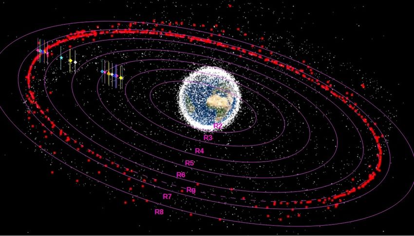
Varela et al.: Planetary magnetospheric response during extreme solar wind conditions

the reconnection region during a Northward inversion of the IMF (Trattner, K. J. et al. 2016). In
addition, the study by Trattner, K. J. et al. (2016) indicates that slow changes in the IMF lead to a
fast response time with respect to the reconnection location, although rapid changes lead to a delay
of several minutes in the reconnection location response. Also, simulations by De Zeeuw, D. L.
et al. (2004) calculated an answer time of around 10 min for the subauroral ionospheric electric
field after a Northward IMF inversion. The relaxation time and magnetosphere dynamics due to
variations of the SW dynamic pressure and temperature were analyzed by Eastwood, J. P. et al.
(2015); Zhang, H. & Zong, Q. (2020); Nishimura, Y. et al. (2020); Shi, Q. Q. et al. (2020), showing
a large variety of transient events that can last from seconds to a hundred of minutes. Consequently,
several response times exist linked to different magnetospheric processes, although in the present
study the main response time is the relaxation time required by the dayside magnetopause to reach
a new equilibrium position, linked to the time required by the Alfvén wave to travel a distance of
the order of the magnetopause standoff distance (Alfvén crossing time). The evolution of the space
weather conditions could be very fast during the impact of the ICME, leading to inversions of the
IMF components as well as local peaks of the SW dynamic pressure and temperature in a few min-
utes. Thus, the relaxation time could be exceeded and the Earth magnetosphere topology shows a
memory regarding previous configurations. Consequently, the simulations performed could over-
estimate the forcing of the SW and IMF because the effect imprinted in the Earth magnetosphere
by previous space weather conditions are not considered.

   The magnetosphere response to the SW and IMF show several interlinked phases that must be
distinguished. First, the response of the day side magnetopause and magnetosheath affecting the
magnetosphere stand off distance, plasma flows toward the inner magnetosphere or the location
of the reconnection regions, between other consequences. Next, the response of the magnetotail,
followed by the ionospheric response and subsequently the ring current response. It should be noted
that the analysis is mainly dedicated to the day side response of the magnetosphere. The analysis of
the magnetotail is not performed in detail, although some implications regarding the magnetic field
at the night side are discussed. On the other hand, the response of the ionosphere and ring current
are out of the scope of the study.

   The IMF and SW parameters are fixed, that is to say, the simulation is assumed complete once
the steady state is reached. Thus, dynamic events caused by the evolving space weather conditions
are not included in the study. The simulations reach the steady state after τ = L/V = 15 code time,
equivalent to t ≈ 16 min of Physical time, although the magnetosphere topology in the Earth day
side is steady after t ≈ 11 min. Consequently, the code can reproduce accurately the magnetosphere
response if the variation of the space weather conditions are roughly steady for time periods of
t = 10 − 15 min.

   The study includes the analysis of the space weather during normal, CME and super-CME
conditions. Table 1 shows the parameter range for each space weather condition:
                                                                             Article number, page 8 of 63
Varela et al.: Planetary magnetospheric response during extreme solar wind conditions

                       Case           n             |v|            T         |B|I MF
                                   (cm)−3        (km/s)         (103 K)        (nT)
                      Normal        ≤ 10          < 500          < 60         ≤ 10
                       CME        [10, 120]    [500, 1000]     [60, 200]    [10, 100]
                      S-CME         > 120        > 1000          > 100        > 100
Table 1. Space weather classification with respect to the SW density, velocity and temperature as well as the
IMF intensity.

    The range of SW and IMF parameters explored in this study exceeds the present space weather
condition for the Earth. The most extreme configurations show the space weather conditions that
could exist during an early period of the Sun main sequence or for the case of an exoplanet mag-
netosphere. Appendix F includes the list of SW and IMF parameters used in the different analysis
performed in section 3.
    In addition, the effect of six different IMF orientations are considered in the study: Earth-Sun
and Sun-Earth (also called radial IMF configurations), Southward, Northward, Ecliptic clockwise
and Ecliptic counter clockwise. Earth-Sun and Sun-Earth configurations indicate an IMF parallel
to the SW velocity vector. Southward and Northward IMF orientations show an IMF perpendicular
to the SW velocity vector at the XZ plane. Consequently, because the tilt of the Earth rotation axis
with respect to the ecliptic plane is included in the model, the simulations show a North-South
asymmetry of the magnetosphere.

3. Effect of the SW and IMF on the Earth / exoplanet magnetosphere topology

Figure 1 shows a 3D view of the system for a Northward IMF orientation. There is an accumulation
of plasma at the planet day side because the SW is slowed down and diverged due to the interaction
with the planet magnetic field, thus the Bow Shock (BS) in the simulations is identified as the
region showing a sudden increase of the plasma density (5 times larger with respect to the SW
density). The SW dynamic pressure bends the planet magnetic field lines (red lines), compressed
on the planet day side and stretched at the nigh side forming the magnetotail. In addition, the
planet magnetic field lines reconnect with the IMF leading to a local erosion/enhancement of the
magnetosphere. The yellow arrows indicate the IMF orientation and the dashed white line the outer
limit of the simulation domain (the star is not included in the model). It should be noted that the
magnetotail can extend more than 100RE although the computation domain is limited to 30RE ,
thus the model only reproduces partially this magnetosphere structure if the SW dynamic pressure
is ≥ 50 nPa and the IMF intensity is ≤ 10 nT. A detail discussion is done in the Appendix C.
    Figure 2 illustrates the effect of the IMF showing the planet magnetic field (red lines), SW
stream lines (green lines), reconnection region (|B| = 10 nT isocontour of the magnetic field, pink
lines), the nose of the BS (vr = 0 isocontour, white lines) and the regions where the magne-
tosheath plasma is injected into the magnetosphere (bold cyan arrows) in the XY plane. We should
clarify that the definition of the magnetosphere reconnection regions is given by the antiparallel
reconnection model, that is to say, the regions with antiparallel magnetic fields. The simulations
                                                                                Article number, page 9 of 63
Varela et al.: Planetary magnetospheric response during extreme solar wind conditions

Fig. 1. 3D view of a typical simulation setup. Density distribution (color scale), Earth magnetic field lines (red
lines) and IMF (yellow lines). The yellow arrows indicate the orientation of the IMF (Northward orientation).
The dashed white line shows the beginning of the simulation domain (note that the star is not included in the
model).

are performed for different IMF orientations, IMF intensities and dynamic pressure values. In the
following, the discussion of the simulation results refers only to the Earth magnetosphere for sim-
plicity, even though some of the configurations analyzed do not correspond to the present space
weather conditions. Such special configurations are highlighted to avoid misunderstanding.
    The simulations show a stronger compression of the magnetosphere as the dynamic pressure
increases leading to a smaller magnetopause stand off distance, see panels a and b. The simula-
tions also shows a large deformation of the Earth magnetosphere if |BI MF | increases. For example,
if |BI MF | increases from 10 to 200 nT for a Northward IMF orientation, see panels c to e, the re-
connection region between the IMF and the Earth magnetic field is located closer to the poles,
enhancing the plasma flows towards the Earth poles. Consequently, the IMF modifies the plasma
injection into the inner magnetosphere, and therefore the plasma flows towards the Earth surface
along the magnetic field lines (bold white arrows). In addition, the magnetosphere is compressed in
the magnetic axis direction and the magnetopause stand off distance decreases. On the other hand,
                                                                                  Article number, page 10 of 63
Varela et al.: Planetary magnetospheric response during extreme solar wind conditions
Fig. 2. Polar cut (XY plane) of the plasma density in simulations with (a) Sun-Earth IMF orientation |BI MF | =
10 nT Pd = 1.2 nPa, (b) Sun-Earth IMF orientation |BI MF | = 10 nT Pd = 30 nPa, (c) Northward IMF
orientation |BI MF | = 10 nT Pd = 1.2 nPa, (d) Northward IMF orientation |BI MF | = 100 nT Pd = 1.2 nPa, (e)
Northward IMF orientation |BI MF | = 200 nT Pd = 1.2 nPa, (f) Southward IMF orientation |BI MF | = 50 nT
Pd = 3 nPa, (g) Earth-Sun IMF orientation |BI MF | = 50 nT Pd = 3 nPa and (h) Ecliptic ctr-cw IMF orientation
|BI MF | = 50 nT Pd = 3 nPa. Earth magnetic field (red lines), SW stream functions (green lines), |B| = 10
nT isocontour of the magnetic field (pink lines) and vr = 0 isocontours (white lines). The bold white arrows
shows the regions where the plasma is injected into the inner magnetosphere.
Southward IMF orientations lead to a magnetic reconnection in the equatorial region that erodes
the Earth magnetic field, causing a decrease of the magnetopause stand off distance and the injec-
tion of SW in the inner magnetosphere at a lower latitude, see panel f. Furthermore, the Earth-Sun
(Sun-Earth) IMF orientation causes a Northward (Southward) displacement at the day side (DS)
and a Southward (Northward) displacement at the night side (NS), see panels a and g. Finally, a
IMF orientation in the Ecliptic plane causes an East/West tilt of the Earth magnetosphere. It should
be noted that the simulations with a SW density of 12 cm−3 and |B|I MF ≤ 60 nT lead to Ma < 1
(vA = 378 km/s if |BI MF | = 60 nT) thus the BS is not formed, consistent with the observations by
Article number, page 11 of 63Varela et al.: Planetary magnetospheric response during extreme solar wind conditions
Lavraud, B. & Borovsky, J. E. (2008); Chane, E. et al. (2012); Lugaz, N. et al. (2016). This is the
case of the simulations shown in the panels d and e.
The deformations induced by the SW / IMF in the Earth magnetosphere during extreme space
weather conditions are very large. Figure 3 show some examples of extreme weather conditions
regarding the IMF intensity, 3d views of the Earth magnetosphere if |B|I MF = 250 nT and Pd = 1.2
nPa for different IMF orientations. The panel (a) indicates a simulation with Sun-Earth IMF, panel
(b) Southward IMF, panel (c) Northward IMF and panel (d) ecliptic ctr-clockwise IMF.
Fig. 3. 3D view of the Earth magnetosphere topology if |B|I MF = 250 nT for (a) a Sun-Earth, (b) Southward,
(c) Northward and (d) ecliptic ctr-clockwise IMF orientations. Earth magnetic field (red lines), SW stream
functions ( green lines) and isocontours of the plasma density for 6 − 9 cm−3 indicating the location of the BS
(pink lines). The blue isocontours indicate the reconnection regions (|B| = 60 nT).
The simulations show that the reconnection regions (blue isocontour of the magnetic field) and
the BS (pink lines of the density isocontour cut with the XZ and XY planes) are located close to
Earth surface (slightly above R/RE = 3), pointing out the decrease of the magnetopause stand off
distance with respect to the simulation with a weaker |BI MF |. The |BI MF | during the impact of an
ICME with the Earth is generally limited to |B|I MF < 100 nT, thus space weather conditions with
|BI MF | = 250 nT falls in the category of super-ICMEs. The simulations indicate how the plasma is
injected inside the inner magnetosphere through the reconnection regions, flowing among the Earth
magnetic field lines from the magnetosheath towards the planet surface (green lines connected with
Article number, page 12 of 63Varela et al.: Planetary magnetospheric response during extreme solar wind conditions
inflow regions at R/RE=2.55 , blue colors). If the IMF is Sun-Earth oriented, the Southward bending
of the magnetosphere at the Earth day side enhances the plasma flows towards the North pole. The
Southward IMF erodes the Earth magnetic field at the Ecliptic plane thus the plasma flows towards
the Equator increase. On the other hand, the Northward IMF erodes the Earth magnetic field near
the magnetic axis promoting the plasma flows towards the Poles. Furthermore, the Ecliptic IMF
orientation induces a West/East tilt in the magnetosphere tilt and the plasma flows towards higher
longitudes.
The simulations, after reaching the steady state, show the formation of a low density and high
temperature plasma belt above the upper ionosphere. The plasma belt, trapped inside the closed
magnetic field lines of the Earth, is generated from two main sources: the solar wind injected into
the inner magnetosphere toward the reconnection regions and a plasma outward flux from the upper
ionosphere to the simulation domain, see figure 4. The plasma belt in the simulations shares some
features with the Van Allen radiation belt (Van Allen, J. A. et al. 1958; Li, W. & Hudson, M.K.
2019) and the Earth’s ring current (Daglis, I.A. 2006; Ganushkina, N. et al. 2017), although it
lacks the complexity of the real magnetosphere structures that cannot be reproduced by a single
fluid MHD model (Hudson, M. K. et al. 1997; Kress, B. T. et al. 2007; Jordanova, V. K. et al.
2014). In addition, the plasma belt narrows as the magnetopause stand off distance decreases, and
is not observed in simulations that reproduce extreme space weather conditions (the plasma belt
is located below R/RE = 2.5). Likewise, other magnetosphere region as the plasmasphere cannot
be correctly reproduced (Singh et al. 2011). Consequently, the analysis of the plasma belt, ring
current and plasmasphere are out of the scope of the present study. It should be noted that these
model limitations can lead to deviations between the simulation results and the observational data
during extreme space weather conditions.
Fig. 4. (a) Polar cut (XY plane) of the plasma temperature and (b) 3D view of the Earth magnetosphere adding
the plasma temperature isocountour T = 26 keV (orange surface, temperature local maxima at R = 3RE planet
day side) and a polar/equatorial (XY / XZ plane) cut of the plasma density for a simulation with no IMF and
Pd = 1.2 nPa. The red lines indicate the Earth magnetic field lines.
Article number, page 13 of 63Varela et al.: Planetary magnetospheric response during extreme solar wind conditions
Summarizing, the correct characterization of the Earth magnetosphere topology with respect to
the IMF intensity and orientation requires a detailed parametric study for regular and extreme space
weather conditions. Such analysis is performed in the following sections, dedicated to calculate the
magnetopause stand off distance, the location of the reconnection regions and the open-close field
line boundary for different IMF intensities and orientations.
3.1. Parametric study of the magnetopause stand off distance
The magnetopause stand off distance R sd could be calculated as the location where the dynamic
pressure of the SW (Pd = m p n sw v2sw /2), the thermal pressure of the SW (Pth,sw = m p n sw v2th,sw /2 =
m p n sw c2sw /γ) and the magnetic pressure of the IMF (Pmag,sw = B2sw /(2µ0 ) are balanced by the
magnetic pressure of the Earth magnetosphere of a dipolar magnetic field (Pmag,E = αµ0 ME2 /8π2 r6 )
and the thermal pressure of the magnetosphere (Pth,MS P = m p n MS P v2th,MS P /2), resulting into the
expression:
Pd + Pmag,sw + Pth,sw = Pmag,E + Pth,MS P (5)
(1/6)
αµ0 ME2
R sd
=
(6)
RE 4π2 m p n sw v2sw + B2sw
+
2m p n sw c2sw
− m p nBS v2th,MS P
µ0 γ
with ME the Earth dipole magnetic field moment, r = R sd /RE and α the dipole compression co-
efficient (α ≈ 2 (Gombosi 1994)). This expression is an approximation and it does not consider
the effect of the reconnection between the Earth magnetic field with the IMF, that is to say, the
approximation assumes a compressed dipolar magnetic field ignoring the orientation of the IMF.
Consequently, the theoretical stand off distance is only valid if |BI MF | is small, thus R sd /RE should
be calculated using simulations for extreme space weather conditions. In the following, the loca-
tion of the magnetopause is defined as the last close magnetic field line at the Earth day side at 0o
longitude in the ecliptic plane. Figure 5 shows the pressure balance in simulations without IMF and
low Pd , large |BI MF | and low Pd as well as large |BI MF | and large Pd .
The simulation without IMF and Pd = 1.2 nPa shows a balance between the dynamic pressure
of the SW and the combined effect of the magnetosphere magnetic and thermal pressure, see panel
a to d of fig 5. The effect of the magnetosphere thermal pressure is important on the pressure
balance for space weather conditions with low |BI MF | and Pd , leading to Pth,MS P /Pmag,E ≈ 1.0.
It should be noted that fig 5, panels (c) and (d), show two local maxima of Pth inside the BS
and nearby the upper ionosphere. The Pth local maxima nearby the upper ionosphere is linked to
the plasma belt (see fig 4), which role on the pressure balance is negligible because the magnetic
pressure generated by the Earth magnetic field in this plasma region is dominant, at least one order
of magnitude higher. For a Northward IMF with |BI MF | = 100 nT and Pd = 1.2 nPa, the leading
Article number, page 14 of 63Varela et al.: Planetary magnetospheric response during extreme solar wind conditions
Fig. 5. Polar cut (XY plane) of the pressure balance. Simulation with no IMF and Pd = 1.2 nPa, isocontour of
(a) Pd , (b) Pmag and (c) Pth . Simulation with Northward |BI MF | = 100 nT and Pd = 1.2 nPa, isocontour of (e)
Pd , (f) Pmag and (g) Pth . Simulation with Northward |BI MF | = 50 nT and Pd = 60 nPa, isocontour of (i) Pd , (j)
Pmag and (k) Pth . Panels (d), (h) and (l) show the total pressure (Ptot = Pd + Pmag + Pmag,sw + Pth ) normalized
to the SW dynamic pressure (isocontour) as well as the isolines of Pd (white line), Pth (green line), Pmag (red
line) and Pmag,sw (pink line), including the respective isoline values (colored characters).
terms in the pressure balance are the magnetic pressure of the IMF (Pd is 3.5 times smaller) and
the magnetosphere magnetic pressure (the magnetosphere thermal pressure is 4 times smaller),
see panels e to h. Consequently, the IMF orientation is particularly important for space weather
conditions with large IMF intensity although low SW dynamic pressure. On the other hand, the
simulation for a Northward IMF with |BI MF | = 50 nT and Pd = 60 nPa indicates a balance between
the magnetic pressure of the magnetosphere (the magnetosphere thermal pressure is 4 − 5 times
smaller) and the combined effect of the SW dynamic pressure and the IMF magnetic pressure, see
panels i to l. In other words, the leading terms of the pressure balance during extreme space weather
conditions are the dynamic pressure of the SW, IMF magnetic pressure and the magnetosphere
magnetic pressure.
We now turn to study the effect of the IMF intensity and orientation on the magnetopause stand
off distance. For this purpose, we will fix the SW parameters to T sw = 1.8 · 105 K and Pd = 1.2
nPa. First, we must clarify that the configurations analyzed are idealizations, that is to say, an IMF
purely oriented towards one direction is rarely observed particularly if the IMF intensity is large.
This subtlety specially applies to the radial IMF configurations, because small deviations on the
ecliptic component breaks the East-West symmetry on the model leading to a substantial variation
of the Earth magnetosphere topology. Nevertheless, all the possible configurations are analyzed for
the completeness of the study, independently of the rarity of the space weather condition. Figure
Article number, page 15 of 63Varela et al.: Planetary magnetospheric response during extreme solar wind conditions
6 shows the location of the magnetopause in the ecliptic plane for different IMF orientations and
intensities.
Fig. 6. Magnetopause stand off distance with respect to |B|I MF if the IMF is oriented in the Sun-Earth direction
(black star), Earth-Sun (red circle), Northward (blue diamond), Southward (green triangle) and Ecliptic ctr-
clockwise direction (pink hexagon). The solid (dashed) lines indicate, for each IMF orientation, the data fit to
the expression R sd /RE = A|B|αI MF of the simulations with Ma > 1 (Ma < 1).
Two different trends are observed in fig 6 for R sd /RE regarding the Ma value of the simulation.
If Ma < 1, simulations with |BI MF | ≤ 60 nT, the pressure balance is dominated by the magnetic
pressure of the IMF and the Earth magnetic field because the BS is not formed, thus the thermal
pressure of the plasma inside the BS does not participate to the balance, see fig 2 panels d and e
as well as fig 5 panels d to f. On the other hand, if Ma > 1, the thermal pressure of the plasma
inside the BS participates in the balance, particularly in the simulations with small |BI MF | values,
see fig 2 panels a and c as well as fig 5 panels a to d (Pth,MS P /Pmag,E ≈ 0.4 − 1.0). The general
trend in the simulations with Ma < 1 indicates a decrease of R sd /RE as the IMF intensity increases
for all the IMF orientations. On the contrary, Ma > 1 simulations for the Sun-Earth and Earth-Sun
IMF orientations show an increase or a constant R sd /RE , respectively. This exception is explained
by the Northward (Southward) bending of the magnetosphere at the planet day side if the IMF is
Earth-Sun (Sun-Earth), see fig 2 panel g, as well as the magnetosphere thermal pressure. The IMF
orientation that leads to the lowest R sd /RE as |BI MF | increases is the Southward orientation while the
Northward IMF orientation leads to the largest R sd /RE . The data for each IMF orientation and Ma
trend is fitted to the expression R sd /RE = A|B|αI MF , indicated by solid lines for the simulations with
Article number, page 16 of 63Varela et al.: Planetary magnetospheric response during extreme solar wind conditions
Ma > 1 and dashed line for the Ma < 1 simulations in figure 6. Table 2 shows the fitting parameters
of the regressions in the simulations with Ma < 1 and Ma > 1 for different IMF orientations.
A α A α
Sun-Earth 220 −0.71 10.9 0.043
±40 ±0.04 ±0.3 ±0.008
Earth-Sun 210 −0.73 11.608 −0.0028
±30 ±0.03 ±0.014 ±0.0004
IMF No BS (Ma < 1) BS (Ma > 1) Northward 35.1 −0.345 16.5 −0.146
±0.9 ±0.005 ±0.9 ±0.017
Southward 33.9 −0.402 16.3 −0.209
±1.4 ±0.009 ±0.7 ±0.014
Ecliptic 22.2 −0.300 18.5 −0.244
±1.3 ±0.013 ±0.9 ±0.016
Table 2. Fit parameters of the regression R sd /RE = A|B|αI MF for different IMF orientations (first column) in
simulations with Ma < 1 (second and third columns) and Ma > 1 (fourth and fifth columns).The standard
errors of the regression parameters are included.
The fit exponent of the simulations with Ma < 1 for Northward, Southward and Ecliptic IMF
orientations are close to the theoretical α = −0.33 value from the equation (6) neglecting the
effect of the SW thermal and dynamic pressure as well as the magnetosphere thermal pressure. The
excursion from the theoretical value is consequence of the IMF orientation, that is to say, due to
the deviation from the dipolar magnetic field assumption. The largest deviation is observed for the
Southward IMF orientation, because the Southward IMF leads to the strongest erosion of the Earth
magnetic field at the day side and the largest decrease of the magnetopause stand off distance. It
should be noted that the exponents are negative because the magnetic pressure of the IMF opposes
to that of the magnetic pressure of the Earth magnetic field. On the other hand, the fit exponents for
the Earth-Sun and Sun-Earth IMF orientations are more than 2 times larger regarding the theoretical
value. The large deviation is explained by the formation of two Alfvén wings at the Earth day and
night side (Chane, E. et al. 2012, 2015). Fig 7, panel a, shows the Alfvén wings formed in the
simulation with Earth-Sun IMF |BI MF | = 250 nT and Pd = 1.2 nPa. The Alfvén wings show the
characteristic bending of the Earth magnetic field near the planet surface, the low velocity plasma
inside the wings and a high velocity plasma linked to the reconnection regions between the IMF
(white lines) and the Earth magnetic field (red lines). The IMF and Earth magnetic field magnetic
pressure, see fig 7 panel b, illustrates the role of the reconnection regions in the pressure balance
and explains the large deviation of the fit exponents from the theoretical value. It must be pointed
out that the Alfvén wings are observed during very special space weather conditions with extremely
low SW densities, that is to say, the simulations performed do not represent the usual conditions
for the formation of the Alfvén wings for the case of the Earth. Nevertheless, the study provides a
generalization of the space weather conditions for the formation of the Alfvén wings in exoplanets
with an Earth-like magnetosphere. The fit exponents of the simulations with Ma > 1 for Northward,
Southward and Ecliptic IMF orientations are smaller regarding the theoretical value because the
effect of the SW dynamic pressure and magnetosphere thermal pressure cannot be neglected. If
|BI MF | increases the magnetosphere thermal pressure decreases because the BS plasma is depleted
Article number, page 17 of 63Varela et al.: Planetary magnetospheric response during extreme solar wind conditions
faster as the reconnection regions are located closer to the Earth surface. Consequently, the pressure
balance of the simulations with |BI MF | ≥ 20 nT are dominated by the SW dynamic pressure and
the combined effect of the magnetosphere thermal pressure and the Earth magnetic field pressure.
Likewise, if |BI MF | > 20 nT, the combination of the SW dynamic pressure and the IMF magnetic
pressure is mainly balanced by the Earth magnetic field pressure. The Earth-Sun and Sun-Earth
IMF orientations show a weak dependency regarding |BI MF |, consequence of the magnetosphere
bending induced by the IMF in conjunction with the thermal pressure of the magnetosphere, almost
unchanged as |B|I MF increases because the BS plasma depletion is rather weak due to the location
of the reconnection region above 12RE . This results in a magnetopause stand off distance that is
nearly constant. In should be noted that the ecliptic clockwise and counter clockwise orientations
lead to the same result.
Fig. 7. Polar cut (XY plane) of the (a) plasma velocity module (color scale) and (b) magnetic pressure. The
red lines indicate the magnetic field lines connected to the Earth surface (red lines) and the white lines the non
reconnect IMF lines.
We are now considering the SW effect on the magnetosphere topology. To this end, IMF pa-
rameters are kept fixed (Sun-Earth IMF orientation with |B| = 10 nT). The IMF intensity in the
simulations is small minimizing the IMF effect on the magnetosphere topology. Figure 8 shows
R sd /RE for different SW densities (fixed T sw = 1.8 · 105 K and |v| = 350 km/s, panel a), SW ve-
locities (fixed T sw = 1.8 · 105 K and n = 12 cm−3 , panel b) and corresponding dynamic pressures
(panel c).
R sd /RE decreases as the SW density or velocity increases, that is to say, a larger dynamic
pressure leads to a stronger compression of the BS. It should be noted that, even if the dynamic
pressure increases up to 160 nPa, extreme space weather conditions comparable to a super-ICME,
R sd /RE > 4.5. Consequently, the direct deposition of the SW toward the Earth surface requires a
large distortion of the magnetosphere by the IMF in addition to the BS compression caused by the
Article number, page 18 of 63Varela et al.: Planetary magnetospheric response during extreme solar wind conditions
Fig. 8. Magnetopause stand off distance with respect to (a) the SW density (fixed v = 350 km/s), (b) SW
velocities (fixed 12· cm−3 ) and (c) dynamic pressure. Sun-Earth IMF orientation with |B| = 10 nT. The pink
stars indicate the magnetopause stand off distance if |B| = 0 nT. The dashed lines indicate the data fit to the
expression R sd /RE = Anα , R sd /RE = A|v|α and R sd /RE = APαd , respectively. The solid red line indicates the fit
line for the data set with n ≤ 60 cm−3 and |v| ≤ 600 km/s. The solid blue line indicates the fit line for the data
set with n > 60 cm−3 and |v| > 600 km/s. The solid pink line indicates the fit line for the data set with n ≤ 60
cm−3 and |v| ≤ 600 km/s and no IMF.
SW dynamic pressure. Again, the data is fitted to the functions R sd /RE = Anα , R sd /RE = A|v|α and
R sd /RE = APαd , respectively. In addition, three different data set are used in the regression, the full
range of values for the SW density and velocity (dashed black line), Pd < 10 nPa cases with n ≤ 60
cm3 and |v| ≤ 600 km/s (red solid line) and Pd > 10 nPa cases with n > 60 cm3 and |v| > 600 km/s
(blue solid line). It should be noted that no plateau is observed in the figures because the minimum
dynamic pressure of the simulations is large enough to induce relatively intense deformation of the
magnetosphere. Table 3 shows the fitting result.
From equation (6), we deduce that the theoretical α exponent is −0.17 for the SW density and
−0.33 for the SW velocity, assuming a negligible effect of the IMF magnetic pressure, SW thermal
pressure and magnetosphere thermal pressure in the pressure balance. The fit exponents are close to
the theoretical exponents once the SW dynamic pressure is large enough (Pd ≥ 10 nPa) to induce a
significant compression of the magnetosphere (R sd /RE < 7), thus the pressure balance is dominated
Article number, page 19 of 63Varela et al.: Planetary magnetospheric response during extreme solar wind conditions
Pd < 10 Pd > 10
(nPa) (nPa)
SW parameter A α A α
Density 17.2 −0.219 12.8 −0.159
±0.4 ±0.007 ±0.3 ±0.004
Velocity 179 −0.491 85 −0.386
±18 ±0.019 ±7 ±0.014
Dynamic pressure 10.60 −0.245 9.0 −0.172
±0.06 ±0.004 ±0.3 ±0.011
Table 3. Fit parameters of the regressions R sd /RE = Anα (first row), R sd /RE = A|v|α (second row) and
R sd /RE = APαd (third row) for the simulations with low (second and third columns) and large (fourth and
fifth columns) Pd . The standard errors of the regression parameters are included.
by the SW dynamic pressure and the magnetic pressure of the Earth magnetosphere, see solid blue
line in figure 8 panels a, b and c. On the other hand, the regression exponents are 25% larger in
the simulations with Pd < 10 nPa, red solid lines in panels a, b and c. The deviation is caused by
the effect of the magnetosphere thermal pressure in the pressure balance. The ratio between the
magnetosphere thermal pressure and the SW dynamic pressure increases from 0.2 to 0.5 if the SW
density decreases from 60 to 6 cm−3 and from 0.4 to 0.8 if the SW velocity decreases from 600
to 100 km/s. Consequently the magnetosphere thermal pressure must be included in the pressure
balance to calculate correctly the magnetopause stand off distance if the SW dynamic pressure is
small. The simulations without IMF (pink stars) and the data fit (pink solid line) indicate the small
effect of the Sun-Earth IMF with |B|I MF = 10 nT in the pressure balance and the Earth magnetic
field topology. The regressions extrapolation indicate a critical Pd ≈ 3.5 · 105 nPa for the direct
deposition of the SW toward the Earth surface, two order of magnitude larger with respect to the
Pd values during super-ICME for the case of the Earth. Consequently, the direct precipitation of
the SW for a relatively weak |B|I MF is extremely unlikely.
Once the effect of the SW on the magnetopause stand off distance is assessed, the following
study is dedicated to the effect of the plasma temperature and dynamic pressure on the thickness of
the BS (Lbs /RE ), with Lbs the distance between the Bow Shock nose and the magnetopause stand
off distance at the ecliptic plane in the day side 0o longitude. An increase of the SW temperature
leads to an increase of the sound speed and the thickness of the BS. On the other hand, a higher
dynamic pressure leads to a compression of the BS. Figure 9 shows the Lbs /RE values calculated
in simulations performed for a range of the SW temperatures (fixed Pd ≈ 2 nPa, panel a) and
the Pd values (fixed T sw = 1.8 · 105 K, panel b). In addition, the data is fitted to the functions
α
Lbs /RE = AT sw and Lbs /RE = APαd , respectively.
The simulations indicate an increase of the BS width of ≈ 0.4RE if the SW temperature raises
from 5 · 104 to 2 · 105 K (panel a). On the other hand, the BS width decreases ≈ 2.8RE if Pd
raises from 0.2 to 160 nPa (panel b). That is to say, the BS compression caused by the SW Pd is
around 6 − 7 times larger with respect to the BS expansion due to the SW temperature. Also, the BS
compression is smaller in the simulations with fixed SW velocity because the plasma temperature
and sound speed inside the BS is higher as well as Pth . In addition, the simulations with Pd < 4
nPa show a weaker dependence between the BS width and Pd (please compare the regression
Article number, page 20 of 63Varela et al.: Planetary magnetospheric response during extreme solar wind conditions
parameters of the simulations with Pd > 4 nPa and Pd < 4 nPa), because the magnetosphere
thermal pressure is comparable to Pd . By contrast, as the simulation Pd increases and the role
of the magnetosphere thermal pressure is less important in the pressure balance, the dependence
between the BS width and Pd increases. It should be mentioned that, the range of SW temperature
and Pd values highlighted includes the typical SW parameters during regular and extreme space
weather conditions (Cliver, E. W. et al. 1990; Mays, M. L. et al. 2015).
In summary, the magnetopause stand off distance calculated in the simulations reveals the key
role of the IMF and SW on the distortion of the Earth magnetosphere for regular and extreme
space weather conditions. The data regressions show clear differences in the pressure balance for
super-Alfvénic and sub-Alfvénic configurations, as well as the important role of the magnetosphere
thermal pressure in the determination of the magnetopause stand off distance if the SW dynamic
pressure and IMF magnetic pressure are low. It should be noted that the range of magnetopause
stand off distance calculated is comparable to the results obtained by other authors (Song, P. et al.
1999; Kabin, K. et al. 2004; Lavraud, B. & Borovsky, J. E. 2008; Ridley, A. J. et al. 2010; Meng,
X. et al. 2012; Wang, J. et al. 2015). Present study contribution entails a larger sample of space
weather configurations thanks to the extended parametric studies performed, as well as the detail
analysis of the topological deformation trends linked to the SW and IMF properties.
3.2. Reconnection region tracking for different IMF orientations and intensities
This section is dedicated to track the location of the reconnection regions for different IMF orien-
tation and intensities. Figure 10 indicates the location of the reconnection regions in the XY plane
for Sun-Earth and Earth-Sun IMF orientations as |BI MF | increases from 10 to 250 nT. Likewise,
figure 11 shows the same study for Northward and Southward IMF orientations. The reconnection
in the simulations is identified as the region where the magnetic field intensity goes to zero.
The reconnection region for the Sun-Earth IMF orientation at the day side moves towards the
South pole as |BI MF | increases, showing a large Northward displacement although smaller in the
Earth-ward direction. On the other hand, the reconnection at the night side moves towards the North
pole and the larger displacement is done in the Sun-ward direction with respect to the Southward
displacement. Regarding the Earth-Sun IMF orientation, the reconnection in the day side moves
Southward towards the North pole although the reconnection in the night side moves toward the
South pole. The differences between the Sun-Earth and Earth-Sun orientations are caused by the
North-South bending of the Earth magnetosphere. It should be noted that the reconnection region
at the night side is located outside the computational domain for the simulations with |BI MF | < 30
nT, thus this data is not included in the analysis.
The reconnection region in the simulations with Southward IMF orientation are located closer
to the equatorial plane and the Earth surface as |BI MF | increases. In the day side, the reconnection
displaces Southward and Earth-ward. Regarding the Northward IMF orientation, the reconnections
are located closer to the poles as |BI MF | increases .The reconnection region at the night side is
Article number, page 21 of 63You can also read