A novel method to identify sub-seasonal clustering episodes of extreme precipitation events and their contributions to large accumulation periods ...
←
→
Page content transcription
If your browser does not render page correctly, please read the page content below

Hydrol. Earth Syst. Sci., 25, 5153–5174, 2021
https://doi.org/10.5194/hess-25-5153-2021
© Author(s) 2021. This work is distributed under
the Creative Commons Attribution 4.0 License.

A novel method to identify sub-seasonal clustering
episodes of extreme precipitation events and their
contributions to large accumulation periods
Jérôme Kopp, Pauline Rivoire, S. Mubashshir Ali, Yannick Barton, and Olivia Martius
Oeschger Centre for Climate Change Research and Institute of Geography, University of Bern, Bern, Switzerland

Correspondence: Jérôme Kopp (jerome.kopp@giub.unibe.ch)

Received: 1 February 2021 – Discussion started: 11 February 2021
Revised: 28 June 2021 – Accepted: 27 August 2021 – Published: 23 September 2021

Abstract. Temporal (serial) clustering of extreme precipi-        1   Introduction
tation events on sub-seasonal timescales is a type of com-
pound event. It can cause large precipitation accumulations       Regional-scale extreme precipitation events can affect the en-
and lead to floods. We present a novel, count-based proce-        tire catchment area of a river or a lake and result in flooding.
dure to identify episodes of sub-seasonal clustering of ex-       Floods can have significant socio-economic impacts such as
treme precipitation. We introduce two metrics to characterise     shortages of drinking water, water-borne diseases, and the
the prevalence of sub-seasonal clustering episodes and their      displacement of people (e.g., IPCC, 2014). The impact of
contribution to large precipitation accumulations. The pro-       catchment-wide precipitation extremes is intensified when
cedure does not require the investigated variable (here pre-      the events happen in close temporal succession, i.e. when
cipitation) to satisfy any specific statistical properties. Ap-   they are serially clustered. The sub-seasonal serial cluster-
plying this procedure to daily precipitation from the ERA5        ing of extreme precipitation is a temporally compounding
reanalysis data set, we identify regions where sub-seasonal       event (Zscheischler et al., 2020), and it is relevant for several
clustering occurs frequently and contributes substantially to     reasons. First, it can lead to floods in rivers and catchment
large precipitation accumulations. The regions are the east       areas with a high retention capacity. Examples include sev-
and northeast of the Asian continent (northeast of China,         eral floods in Lake Maggiore in southern Switzerland (Bar-
North and South Korea, Siberia and east of Mongolia), cen-        ton et al., 2016), the floods in England in winter 2013/2014
tral Canada and south of California, Afghanistan, Pakistan,       (Priestley et al., 2017), the floods in Pakistan in 2010 (e.g.,
the southwest of the Iberian Peninsula, and the north of Ar-      Lau and Kim, 2012; Martius et al., 2013), and the floods
gentina and south of Bolivia. Our method is robust with re-       in China in summer 2020 (Guo et al., 2020). Second, the
spect to the parameters used to define the extreme events (the    short recovery time between events can overburden rescue
percentile threshold and the run length) and the length of the    and response teams and prevent proper clean-up and efficient
sub-seasonal time window (here 2–4 weeks). This procedure         repairs to damaged protective structures (Raymond et al.,
could also be used to identify temporal clustering of other       2020). Therefore, temporal dependence of precipitation and
variables (e.g. heat waves) and can be applied on different       other extremes is of interest for insurance companies (Priest-
timescales (sub-seasonal to decadal). The code is available at    ley et al., 2018) as floods are a major cause of financial
the listed GitHub repository.                                     loss from natural hazards (European Environment Agency,
                                                                  2020).
                                                                     A number of previous studies have analysed the statistical
                                                                  properties of the serial clustering of extreme events. Mailier
                                                                  et al. (2006), Vitolo et al. (2009) and Pinto et al. (2013) stud-
                                                                  ied European winter storms (see Dacre and Pinto, 2020, for
                                                                  a review); Villarini et al. (2011) quantified clustering of ex-

Published by Copernicus Publications on behalf of the European Geosciences Union.
5154                                                                     J. Kopp et al.: Serial clustering of heavy precipitation

treme precipitation in the North American Midwest; and Vil-        2     Data and methods
larini et al. (2012) focused on extreme flooding in Austria. In
these studies, clustering in time was assessed using the index     2.1    Catchment selection and precipitation aggregation
of dispersion (variance-to-mean ratio) of a one-dimensional
homogeneous Poisson process model, i.e. a Poisson process          This study uses precipitation from the ERA5 reanalysis data
with a constant rate of occurrence (Cox and Isham, 1980).          set (Hersbach et al., 2020) by the European Centre for
Villarini et al. (2013) analysed flood occurrence in Iowa us-      Medium-Range Weather Forecasts (ECMWF). The precip-
ing a Cox regression model, i.e. a Poisson process with a          itation fields are interpolated to a 0.25◦ × 0.25◦ spatial grid,
randomly varying rate of occurrence (e.g., Cox and Isham,          and the hourly precipitation is aggregated to daily precipita-
1980; Smith and Karr, 1986). Yang and Villarini (2019) also        tion for the period 2 January 1979 to 31 March 2019. Pre-
used a Cox regression model to show that heavy precipita-          cipitation is not directly constrained by observations in the
tion events over Europe exhibit serial clustering. Their study     ERA5 reanalysis data set as it stems from short-range nu-
also indicated that reanalysis products are skilful in repro-      merical weather model forecasts. Consequently, the quality
ducing serial clustering identified in observations. Barton        of the precipitation data depends on the forecast quality.
et al. (2016) studied serial clustering of extreme precipita-         For catchment boundaries we use the HydroBASINS data
tion events in southern Switzerland using Ripley’s K func-         set format 2 (with inserted lakes) (Lehner and Grill, 2013).
tion (Ripley, 1981) applied to a one-dimensional time axis         HydroBASINS contains a series of polygon layers that de-
(Dixon, 2002).                                                     lineate catchment area boundaries at a global scale. This
    All studies discussed above used statistical models to iden-   dataset has a grid resolution of 15 arcsec, corresponding to
tify significant serial clustering of extreme events. However,     approximately 500 m at the Equator. The HydroBASINS
none of those methods are able to directly identify individ-       product provides 12 levels of catchment area delineations.
ual clustering episodes. According to the review of Dacre          The first three levels are assigned manually, with Level 1 dis-
and Pinto (2020), there are no widely used impact metrics          tinguishing nine continental regions. From Level 4 onward,
used as a proxy for precipitation-related damage, and only         the breakdown follows a Pfafstetter coding, where a larger
a recent study by Bevacqua et al. (2020) introduced a count-       basin is sequentially subdivided into nine smaller units: the
based procedure to identify individual cyclone clusters, com-      four largest tributaries and the five inter-basins. A basin is di-
bined with an impact metric based on precipitation accumu-         vided into two sub-basins at every location where two river
lations. Here we propose a novel count-based procedure to          branches meet and where they have an individual upstream
study serial clustering of catchment-aggregated heavy pre-         area of at least 100 km2 . We use Level 6 of HydroBASINS
cipitation using daily precipitation data from ERA5 (Hers-         for our study. This choice is motivated further below.
bach et al., 2020). We investigate sub-seasonal serial clus-          Daily precipitation aggregated by catchment area was
tering of extreme precipitation events in the mid-latitudes of     computed by taking the average of all ERA5 grid point values
the Northern Hemisphere and Southern Hemisphere. We also           located within the catchment area (see Fig. 1 for an illustra-
quantify the contribution of sub-seasonal serial clustering to     tion). Computations were performed using the GeoPandas
large sub-seasonal precipitation accumulations at the catch-       (version 0.6.0 and onward) Python library (Jordahl et al.,
ment level. More specifically, we address the following ques-      2019). Some small or elongated catchments had few or no
tions. (1) Globally, what are the regions (catchments) where       grid points inside their boundaries. This is a consequence of
sub-seasonal serial clustering of extreme precipitation occurs     the Pfafstetter coding used to construct the HydroBASINS
frequently? (2) What is the contribution of sub-seasonal clus-     division, where large differences can exist in the catch-
tering to large sub-seasonal (14 to 28 d) precipitation accu-      ment areas for a given level. We retained only catchments
mulations? (3) Are the results affected by the choice of the       containing at least five ERA5 grid points for our analy-
parameters used to identify the extreme events and the length      ses. The choice of HydroBASINS Level 6 and the removal
of the period (sensitivity analysis)?                              of the smallest catchments allow us to focus our analysis
    The paper is organised as follows: the data and methods        on relatively large catchments (90 % of the catchments are
are introduced in Sect. 2. The results are presented and dis-      3000 km2 or larger). Such large catchments are sensitive to
cussed in Sect. 3. Finally, general conclusions and future re-     extended periods of heavy rainfall lasting for several days
search avenues are presented in Sect. 4. All important quan-       or longer (Westra et al., 2014), and consequently the impact
tities used in this study are listed in Table 1.                   of subseasonal clustering is likely to be more important for
                                                                   those catchments.
                                                                      Further, we kept only catchments located in two latitudi-
                                                                   nal bands between 20 and 70◦ with a catchment 99th an-
                                                                   nual percentile (99 p) of daily precipitation above 10 mm
                                                                   (Fig. 2). Those criteria remove catchments from the tropics
                                                                   and the poles as well as dry areas and result in the selection of
                                                                   6466 catchments. The timing of extreme precipitation (time

Hydrol. Earth Syst. Sci., 25, 5153–5174, 2021                                        https://doi.org/10.5194/hess-25-5153-2021
J. Kopp et al.: Serial clustering of heavy precipitation                                                                                      5155

Table 1. Symbols for important quantities used in this study.

  Symbol     Definition
  r          Run length parameter (minimal distance between two high-frequency clusters)
  t          Threshold (above which daily precipitation is considered an extreme event)
  w          Time window length (duration of a sub-seasonal clustering episode)
  nw         Count of extreme events (resulting from the runs declustering) during a time window of w days
  accw       Precipitation accumulation during a time window of w days
  Nep        Number of sub-seasonal clustering episodes considered in the classifications
  Cln        Classification of sub-seasonal clustering episodes with the highest extreme event counts and the largest precipitation accumulations
  Clacc      Classification of sub-seasonal clustering episodes with the largest precipitation accumulations
  qi         Weight of the ith episode in a classification
  Scl        Clustering metric
  Sacc       Accumulation metric
  Scont      Contribution metric
  φ̂         Estimator of the index of dispersion

                                                                            pared moderate to extreme daily precipitation from ERA5
                                                                            against two observational gridded datasets, EOBS (station-
                                                                            based) and CMORPH (satellite-based). Using the hit rate as
                                                                            a measure of co-occurrence, they found that for days exceed-
                                                                            ing the local 90th percentile, the mean hit rate is 65 % be-
                                                                            tween ERA5 and EOBS (over Europe) and 60 % between
                                                                            ERA5 and CMORPH (globally). They also found that the
                                                                            differences between ERA5 and CMORPH are largest over
                                                                            NW America, central Asia, and land areas between 15◦ S
                                                                            and 15◦ N (the tropics). Another recent study by Tuel and
                                                                            Martius (2021) on sub-seasonal clustering compared ERA5
                                                                            with three satellite-based datasets (TRMM, CMORPH and
Figure 1. Example of a catchment area (Aare basin, Switzerland in
                                                                            GPCP), as well as output from 25 CMIP6 global climate
green). The red lines show the HydroBASINS Level 6 catchment
area division. The blue dots indicate the ERA5 grid points. Country
                                                                            models (GCMs). They found a good agreement on the spatio-
borders are indicated by black lines.                                       temporal clustering patterns across datasets.

                                                                            2.2    Identification of extreme precipitation events

of the year) is important for the present study because our                 We used a peak-over-threshold approach to identify extreme
method is based on counting how many extreme events hap-                    precipitation events from the time series of daily precipi-
pen in a certain time window (see Sect. 2.3). Rivoire et al.                tation per catchment (Coles, 2001). We consider only the
(2021) showed that this timing of extreme precipitation is                  precipitation values exceeding the local annual 99th per-
well captured by ERA5 in the extratropics but less so in the                centile. We use annual percentiles rather than seasonal per-
tropics. Our choice of ERA5 was also motivated by its global                centiles because they are more impact relevant. To anal-
coverage, its regular spatial and temporal resolution, and its              yse sub-seasonal serial clustering, high-frequency cluster-
consistency with the large-scale circulation (Rivoire et al.,               ing had to be removed from the daily precipitation time se-
2021).                                                                      ries. High-frequency clustering, i.e. successive days of ex-
   Our method can be applied to any kind of dataset, inde-                  treme precipitation, can be caused by a stationary synop-
pendently of their spatial configuration and temporal reso-                 tic system (e.g., an extratropical cut-off cyclone). We em-
lution. Still, we do not expect our results to change signif-               ployed the “runs declustering” method to account for the
icantly using other gridded datasets, surface station data or               high-frequency clustering (Ferro and Segers, 2003). Thereby,
satellite observations. Indeed, previous studies have shown                 given a run length r and a threshold t, days with precipita-
that precipitation extremes in gridded observational and re-                tion exceeding t that are separated by fewer than r days with
analysis datasets correlated significantly (Donat et al., 2014)             precipitation below t were grouped into one high-frequency
and that reanalysis products tended to agree in capturing the               cluster (see Fig. 3a for an illustration). The run declustering
temporal clustering of heavy precipitation (Yang and Vil-                   successively removes the short-term temporal dependence of
larini, 2019). These studies used ERA-Interim, the prede-                   extremes so as to focus exclusively on clustering at longer
cessor of ERA5. More recently, Rivoire et al. (2021) com-                   timescales (weekly and above). In this framework, a multi-

https://doi.org/10.5194/hess-25-5153-2021                                                  Hydrol. Earth Syst. Sci., 25, 5153–5174, 2021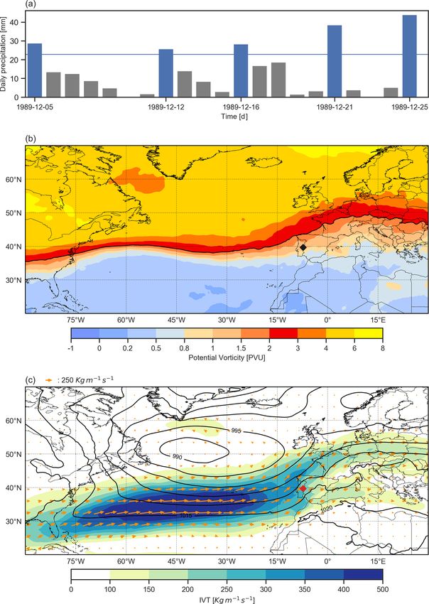
5156                                                                        J. Kopp et al.: Serial clustering of heavy precipitation

Figure 2. The 99th annual percentile of daily precipitation per catchment (mm d−1 ). White areas correspond to the catchments that have
been excluded from the analysis.

day sequence of afternoon severe convective storms at the             of the high-frequency clusters with the run declustering de-
same grid point would be reduced to a single event, while             scribed above.
being composed of multiple independent events. This is not
an issue because the present research is more targeted at the         2.3    Identification of sub-seasonal clustering episodes
larger-scale structures, such as mid-latitudes cyclones and
cut-off lows. More importantly, the spatial (0.25◦ lat–long)
and temporal (daily) resolutions of ERA-5 are too coarse to           The identification of sub-seasonal clustering episodes is
properly target convective-scale precipitation, and many con-         equivalent to searching for time periods (here 2 to 4 weeks)
vective extremes would be missed. Input data with a higher            that contain several extreme precipitation events. The first
temporal and spatial resolution should be used to apply our           step is to count the number of independent extreme precip-
approach to shorter timescales. After applying the decluster-         itation events (nw ) in a running (leading) time window of
ing approach, a series of binary events of extreme daily pre-         w days, after the run declustering has been applied to the
cipitation was defined (Fig. 3a and b). In the case of a high-        time series. This count is computed for each day of the time
frequency cluster, the first day of the cluster was retained as       series over the next w−1 d (not w, as the starting day is in-
the representative day for the event.                                 cluded in the time window length). In parallel, we calculate
   The choice of the two parameters (t and r) affects the dis-        the running sum of daily precipitation (accw ) over the same
tribution of independent extreme events (Coles, 2001). We             leading time window w. Time windows of w = 14, 21 and
followed the empirical approach of Barton et al. (2016) to            28 d were investigated. Figure 3c and d show the values of
determine reasonable values for the parameters. First, we se-         n21 and acc21 , corresponding to the time series of Fig. 3a.
lected two different thresholds: the 98th and 99th annual per-           We then run an automated clustering episode identifica-
centiles (further denoted as 98 p and 99 p) of the catchment          tion algorithm that consists of the following steps: (i) iso-
area daily precipitation distribution. These thresholds have          late the days with the largest value of nw (highlighted in
been used in previous studies (e.g. Fukutome et al., 2015).           red in Fig. 3c). (ii) Among these days, retain the one with
   The run length can either be determined with an objective          the largest accumulation accw (the purple bar in Fig. 3d).
method (Barton et al., 2016; Fukutome et al., 2015) or chosen         This selects a clustering episode which starts at the retained
based on meteorological process arguments (Lenggenhager               day and ends w − 1 d later (shown by the red rectangle in
and Martius, 2019). Following the approach of Lenggen-                Fig. 3a). The clustering episode identified in Fig. 3a contains
hager and Martius (2019), we tested run lengths of both 1             four extreme events (n21 = 4), and the related accumulation
and 2 d, corresponding to the influence time of a cyclone at          acc21 is 275 [mm]. (iii) Reduce the time series by remov-
one location (Lackmann, 2011).                                        ing all days within w−1 d before and after the starting day
   The R package evd (Stephenson, 2002) was used for the              of the selected episode (the purple window in Fig. 3d), to
computation of the yearly percentiles and the identification          avoid further selected episodes from overlapping. (iv) Repeat
of independent peaks over the threshold, i.e. for the removal         steps (ii) and (iii) on the reduced time series to successively
                                                                      select the next episodes with the largest values of nw and
                                                                      accw until a predetermined number of episodes Nep = 50 is

Hydrol. Earth Syst. Sci., 25, 5153–5174, 2021                                           https://doi.org/10.5194/hess-25-5153-2021
J. Kopp et al.: Serial clustering of heavy precipitation                                                                              5157

reached. The choice of Nep is discussed below in greater de-
tail, and at this stage we emphasise that limiting the selec-
tion to 50 episodes is sufficient for our method. This iterative
selection results in the identification of 50 non-overlapping
clustering episodes sorted by the number of extreme events
(nw ) and then by accumulations (accw ). We denote this clas-
sification as Cln . The left panel of Table 2 shows the Cln
classification obtained for a subcatchment of the Tagus river
in the Iberian Peninsula (HydroBASINS ID: 2060654920).
The Cln classification contains information about the fre-
quency of sub-seasonal clustering. In a catchment where sub-
seasonal clustering scarcely happens, Cln would typically be
composed of a majority of episodes having a small number
of extremes (e.g. nw ≤ 2). However, for a catchment where
sub-seasonal happens frequently, Cln would be composed of
several episodes with more extreme events (e.g. 2 ≤ nw ≤ 6).
Additional examples of catchments can be found in Ap-
pendix A.
   In addition, we identify and classify the episodes with
the largest precipitation accumulations as follows: we ap-
ply steps (ii) to (iv) of the automated identification algorithm
to the accumulation time series. This is equivalent to select-
ing episodes using the sole criterion of maximising accw (the
21 d accumulations) at each iteration. This second selection
results in the identification of 50 non-overlapping episodes
sorted by accumulations (accw ). We denote this classifica-          Figure 3. Schematic illustration of the identification of a sub-
tion as Clacc . The right half of Table 2 shows the Clacc clas-      seasonal clustering episode with w = 21 d. (a) Time series of daily
sification obtained for the same catchment as the left half.         precipitation with extreme precipitation days marked by blue bars;
All episodes listed in Table 2 are represented on the yearly         the horizontal blue line represents the threshold t (e.g. the 99th per-
timeline of Fig. 4 (in orange for Cln , in blue for Clacc and in     centile) defining the extreme events; the light blue shading high-
grey when they overlap), along with the timing of all extreme        lights a high-frequency cluster (r = 2 d), and the red rectangle de-
events (black dots). We note that the choice of a centred or         notes the clustering episode identified using the information of pan-
lagged window, instead of a leading window, does not change          els (c) and (d). (b) Series of binary events of extreme precipita-
the values of nw and accw , except for the first and last w days     tion obtained after applying the declustering approach to the daily
                                                                     precipitation. (c) Number of extreme precipitation events in a run-
of the time series. This has no significant impact on the re-
                                                                     ning (leading) time window of 21 d (n21 ) based on the time series
sults.                                                               in panel (b); the light red shading indicates the day with the largest
   The degree of similarity between Cln and Clacc is the key         n21 . (d) Precipitation accumulation in a running (leading) time win-
point in our method to evaluate the contribution of clustering       dow of 21 d (acc21 ) derived from the time series of panel (a); the
to large accumulations. This degree of similarity can be eval-       purple bar denotes the day with the largest acc21 among the days
uated by doing a rank-by-rank comparison of the number of            with highest n21 ; this day is the starting day of the selected clus-
extreme events (nw ) in the episodes of Cln with the episodes        tering episode; all days within the light purple shading are removed
of Clacc . If the episodes composing Clacc and Cln have the          from the initial time series in the next step of the selection algo-
same nw at each rank, then it means that the episodes with           rithm.
the largest number of extreme events are also leading to the
largest accumulations. In this particular case, the contribution
                                                                     it means that the episode is not present in the other classifi-
of clustering to accumulations is maximised. If an episode
                                                                     cation. In this example, both classifications share the same
of Clacc has fewer extreme events than the episode with the
                                                                     first episode (nw = 5), but their second and third episodes
same rank in Cln , then the contribution of clustering to accu-
                                                                     have different nw . We also note one episode without extreme
mulations is below the maximum contribution. The episodes
                                                                     events in Clacc at rank 11. The additional examples in Ap-
selected in Cln and Clacc can be the same and ordered simi-
                                                                     pendix A illustrate cases with different degrees of similarity
larly or differently (they appear in grey in Fig. 4), but they can
                                                                     between Cln and Clacc .
also differ (they appear in orange or blue in Fig. 4). The fifth
columns of the left and right halves in Table 2 illustrate such
a comparison, where the corresponding rank of each episode
in the other classification is displayed. If the column is empty,

https://doi.org/10.5194/hess-25-5153-2021                                          Hydrol. Earth Syst. Sci., 25, 5153–5174, 2021
5158                                                                            J. Kopp et al.: Serial clustering of heavy precipitation

Table 2. First 15 episodes of the Cln (left half) and Clacc (right half) classifications for the catchment with HydroBASINS ID 2060654920.
Episodes of Cln (Clacc ) are ranked according to their number of extreme events n21 (their accumulation acc21 ). The rightmost column of
each panel indicates the corresponding rank of the episode in the other classification; if it is empty, the episode is not present in the other
classification.

                                         Cln                                                      Clacc
                Rank     Starting day           acc21    n21    Rank     Rank      Starting day           acc21   n21    Rank
                Cln                             [mm]            Clacc    Clacc                            [mm]            Cln
                1        5 December 1989         281       5        1        1     5 December 1989         281      5        1
                2        25 December 1995        275       4                 2     19 December 1995        279      3
                3        23 December 2009        213       4                 3     16 October 2006         275      2       11
                4        25 January 1979         247       3        5        4     27 February 2018        255      2       12
                5        11 November 1989        242       3        6        5     25 January 1979         247      3        4
                6        4 December 1996         229       3        7        6     11 November 1989        242      3        5
                7        3 October 1979          188       3       16        7     4 December 1996         229      3        6
                8        19 October 1997         188       3                 8     16 December 2009        220      3
                9        18 October 2012         161       3                 9     21 December 2000        214      2       13
                10       25 October 2011         141       3                10     2 November 1983         212      2       14
                11       16 October 2006         275       2        3       11     15 February 2010        202      0
                12       27 February 2018        255       2        4       12     14 December 1981        196      1       28
                13       21 December 2000        214       2        9       13     1 November 1997         191      2
                14       2 November 1983         212       2       10       14     20 November 2000        191      2       15
                15       20 November 2000        191       2       14       15     13 January 1996         190      2

                                                                          2.4    Metrics for sub-seasonal clustering

                                                                          Next we define metrics that synthesise the properties of
                                                                          the two classifications to compare catchments. An intuitive
                                                                          choice for the metrics would be to average the number of ex-
                                                                          treme events; however such a choice would result in a loss of
                                                                          information (see Appendix C for a more detailed discussion
                                                                          on this). We take a different approach, equivalent to defining
                                                                          a scoring system, where each episode is given a weight qi
                                                                          depending on its rank in the classification, and this weight
                                                                          is used as a proportion factor for the number of extreme
                                                                          events in the episode. We have many options for defining
                                                                          the weights. For example, taking the average over the Nep
                                                                          episodes (as discussed in Appendix C) is the same as set-
                                                                          ting all weights equal to N1ep . Sitarz (2013) discusses a math-
                                                                          ematical approach for defining a scoring system in sports,
Figure 4. For the catchment 2060654920, all extreme events are            with two intuitively appealing properties. First, the first place
shown as black dots, and 21 d episodes are highlighted by the             should be rewarded more points than the second, and the sec-
coloured rectangles. Episodes appearing in both classifications are       ond more than the third, and so on. In our case, rewarding
shown in grey, and those appearing only in the Cln classification         more points is equivalent to giving a larger weight. Second,
are shown in orange, whereas those only in the Clacc classifica-          the difference between the ith place and the (i + 1)th should
tion are shown in blue. Episodes containing two or more extreme
                                                                          be larger than the difference between the ith place and the
events (nw ≥ 2) are highlighted with a red edge. The clustering
and contribution metrics (see Sect. 2.4) for this catchment are re-
                                                                          (i + 2)th. The second property means that someone gaining a
spectively Scl = 43.63 and Scont = 0.89, indicating prevalent sub-        place (or a rank) should be rewarded more if the initial rank
seasonal clustering with a substantial contribution to large accumu-      is higher, as improving at upper ranks is more challenging
lations (similar to the catchment of Appendix A1).                        than improving at lower ranks. We then follow the method of
                                                                          the incentre of a convex cone (Sitarz, 2013) to construct our
                                                                          weighting scheme (see Appendix B for a detailed descrip-
                                                                          tion). The same weight qi is assigned to the ith episode of
                                                                          each classification (Cln and Clacc ). We have tried two other

Hydrol. Earth Syst. Sci., 25, 5153–5174, 2021                                                https://doi.org/10.5194/hess-25-5153-2021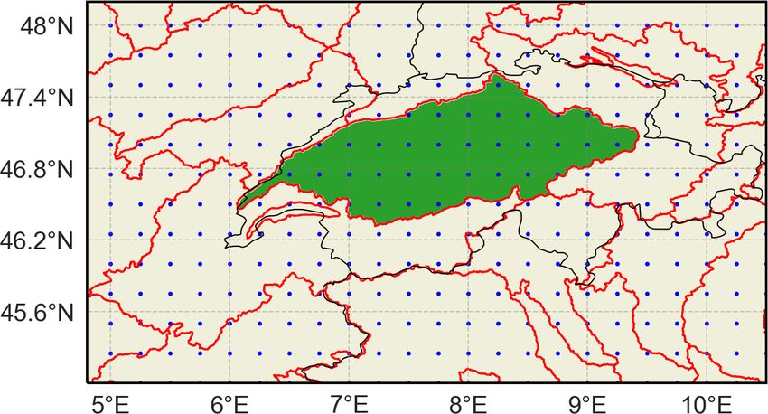
J. Kopp et al.: Serial clustering of heavy precipitation                                                                       5159

weighting schemes, also satisfying the two required proper-         ples of catchments having high and low values of Scont as an
ties: the inverse of the rank (qi = 1i ) and the inverse of the     illustration.
square root of the rank (qi = √1 ). The former gave slightly           We now briefly address some technical points related to
                                  i
too much weight to the very first episodes of the classifica-       the definition of the metrics. First, we note that performing a
tion, and the latter gave almost identical results to the incen-    regression between Cln and Clacc would be a more conserva-
tre method. Our results are hence only slightly sensitive to        tive approach in assessing their degree of similarity because
the choice of the weighting scheme, as long as it satisfies the     it would require giving a unique identifier to each episode
two desired properties.                                             according to its starting day. In that case, the strength of the
   We can now use each weight qi as a proportion factor             regression would be lowered when two episodes containing
for the corresponding number of extreme events in the ith           the same number of extreme events just swap their ranks in
episode for both classifications and derive the three follow-       the two classifications. Such a change does not affect Scont .
ing metrics.                                                           Second, both scores depend on the number of clustering
                                                                    episodes considered (Nep ). The choice of Nep is arbitrary
          X                                                         but should be guided by some principles. The same value of
  Scl =           nw (i) · qi                                (1)    Nep should be chosen for both Scl and Sacc and for all catch-
          i∈Cln                                                     ments to allow for comparisons. This implies that one cannot
                                                                    simply iterate over the precipitation time series until all non-
           X
Sacc =              nw (i) · qi                              (2)
          i∈Clacc                                                   overlapping episodes have been selected and classified. By
          Scl                                                       doing so, one could end up with different values of Nep for
Scont =                                                      (3)    each catchment. Moreover, the contribution of the ith term to
          Sacc
                                                                    the sums in Scl and Scont becomes smaller as Nep increases.
   The first metric Scl , called the clustering metric, is the      We have tested several values of Nep ranging from 10 to 50
weighted (qi ) sum of the number of extreme events (nw (i))         and found that the results with Nep ranging from 30 to 50 are
over all episodes (i = 1 to 50) in the Cln classification. Scl is   comparable. Hence, we selected Nep = 50 for our analysis.
proportional to the number of extreme events in the cluster-           Third, Scl and Sacc both increase with the number of ex-
ing episodes. It is most sensitive to the number of extreme         treme events per episode, so any parameter change which in-
events in the first clustering episodes, which are given the        creases this number will also lead to an increase in Scl and
largest weight. In Sect. 2.5, we show that Scl correlates well      Sacc . The variations in Scont with the parameters depend on
with the index of dispersion – a widely used measure of clus-       the variations in both Scl and Sacc . This sensitivity to the pa-
tering. Appendix A provides examples of catchments with             rameters is assessed in Sect. 3.2.
high and low values of Scl for illustration.
   The second metric Sacc , called the accumulation metric,         2.5     Correlations with index of dispersion and
is computed similarly to Scl , but using the episodes of the                significance test
Clacc classification, where episodes were ranked according
to their accumulations. As Scl and Sacc are computed using          We computed the index of dispersion φ for each catchment
the same weights, their ratio Scont can be used to make a           (Cox and Isham, 1980; Mailier et al., 2006) to compare our
rank-by-rank comparison. Scont is equal to 1 when Sacc = Scl ,      results to a more traditional method. For an homogeneous
i.e. when the two classifications have episodes with the same       Poisson process, φ = 1. When φ > 1, the process is more
number of extreme events at identical ranks. Scont is equal         clustered than random. When φ < 1, the process is more reg-
to 0 when Sacc = 0, i.e. when all episodes in the Sacc classi-      ular than random (Mailier et al., 2006). To estimate φ for a
fication contain no extreme events (nw (i) = 0 ∀i ∈ [1, Nep ]).     given catchment, we separated the precipitation time series
In this particular case, subseasonal clustering does not con-       in successive intervals of w days and counted the number of
tribute to large accumulation, and there is even no contri-         extreme events in each interval. An estimator of φ is then
bution of single extremes to large accumulations. In other          given by (Mailier et al., 2006)
cases, a proper assessment of the contribution of clustering               sn2
to large accumulations is done by considering both Scl and          φ̂ =       ,                                                 (4)
                                                                           n
Scont . Scont alone evaluates the similarity of the two classi-
fications, and catchments can have low values of Scl (lim-          where n is the sample mean and sn2 the sample variance of
ited sub-seasonal clustering) and high values of Scont at the       the number of extreme events in the 14199w    intervals, where
same time. The exact interpretation of intermediary values of       14199 is the number of days in our time series.
Scont requires looking at both classifications (Cln and Clacc )        We computed Scl and φ̂ and calculated their Spearman
in detail to see where they differ from each other. For ex-         rank correlation coefficient (Wilks, 2011) for all catchments
ample, if Scont = 0.8, both classifications have a high degree      and for each parameter combination (Table 3). All correla-
of similarity, but it does not necessarily imply that 80 % of       tion coefficients are positive with values between 0.738 and
the episodes are ranked equally. Appendix A provides exam-          0.885 and significant with p values < 10−5 . Figure 5 displays

https://doi.org/10.5194/hess-25-5153-2021                                          Hydrol. Earth Syst. Sci., 25, 5153–5174, 2021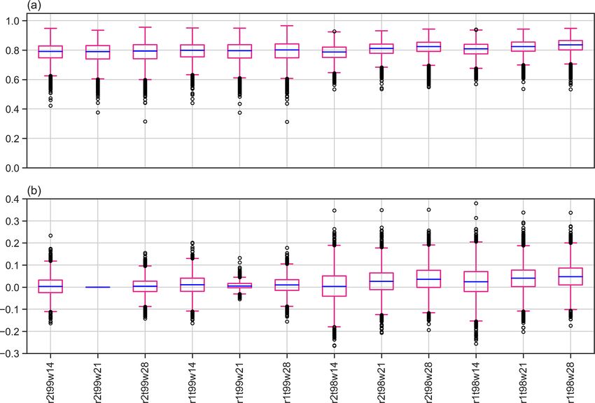
5160                                                                     J. Kopp et al.: Serial clustering of heavy precipitation

a scatter plot of Scl versus φ̂ for all catchments for the ini-    Table 3. Spearman rank correlation coefficients between Scl and φ̂
tial parameter combination (r = 2 d, t = 99 p, w = 21 d) and       for all parameter combinations.
illustrates this correlation. This significant positive correla-
tion means that the use of Scl and φ̂ leads to similar con-                          r          t       w     Cor.
clusions about the clustering of extreme precipitation events.                       [days]   [p]   [days]   coeff.
This is further illustrated in Figs. 6a and E1, which respec-
                                                                                     1        98        14    0.832
tively show a map of Scl and a map of φ̂ for the initial pa-                         1        98        21    0.871
rameter combination. A visual comparison of the two maps                             1        98        28    0.885
reveals that regions of high (low) Scl correspond to regions                         1        99        14    0.814
of high (low) φ̂.                                                                    1        99        21    0.844
   An evident drawback of Scl compared to φ̂ is the lack of                          1        99        28    0.860
a reference value above (below) which there is (no) cluster-                         2        98        14    0.738
ing (e.g. φ̂ = 1). While we cannot derive such a reference                           2        98        21    0.816
value, we can still use a bootstrap-based approach to assess                         2        98        28    0.840
how significant the value of Scl is for each catchment. More                         2        99        14    0.765
                                                                                     2        99        21    0.816
precisely, we tested the following hypothesis:
                                                                                     2        99        28    0.836

H0 : The clustering episodes contain a number of extreme
   precipitation events (nw ) which is not higher than for a
   distribution of those extremes without temporal struc-          two selection methods for the initial parameter combination
   ture (random).                                                  and found only limited differences.
                                                                      Many catchments have a very low p value because we take
H1 : The clustering episodes contain a number of extreme           an annual percentile for defining the extreme precipitation
   precipitation events (nw ) which is significantly higher        events. With this definition, catchments with strong season-
   than for a distribution of those extremes without tempo-        ality in the precipitation (e.g. with extremes occurring during
   ral structure (random).                                         a “wet” season) will have their extreme events occurring only
                                                                   during a few months. A random permutation of the daily pre-
   We reject H0 if the observed value of Scl is significantly      cipitation will redistribute the extremes equally during the
greater than a given threshold. A rejection of H0 at a certain     year in most cases, corresponding to much lower values of
level of significance will be further noted as “significant sub-   Scl . Taking seasonal percentiles would most likely result in
seasonal clustering” for simplicity. To this end, 1000 random      fewer catchments having very low p values. The implica-
samples were generated by doing permutations of the pre-           tions of seasonality and the choice of an annual percentile
cipitation time series (i.e. each daily value is drawn only one    are further discussed in Sect. 4.
time in each sample, without repetition; this way the distribu-
tion quantiles remain identical.). Scl was calculated for each     3     Results
sample, using the initial parameter combination and leading
to an empirical distribution of Scl values. An empirical cu-       3.1    Sub-seasonal clustering and its contribution to
mulative distribution function (ECDF) was calculated from                 accumulations
the Scl empirical distribution, and an empirical p value was
obtained by evaluating the ECDF at the observed Scl value:         Sub-seasonal clustering is prevalent in catchments having
1 − ECDF(Scl (obs)). At a 1 % level, approx. 42 % of the           high values of Scl (see Sect. 2.5). Such catchments are lo-
catchments (2729 out of 6466) show significant sub-seasonal        cated in the east and northeast of the Asian continent (north-
clustering (Fig. 6b, catchments in red).                           east of Siberia, northeast of China, Korean Peninsula, south
   Interestingly, the whole Scl empirical distribution based on    of Tibet), between the northwest of Argentina and the south-
the random samples is almost identical for all catchments,         west of Bolivia, in the northeast and northwest of Canada as
with a mean value around 31.42. This means that a selec-           well as in Alaska, and in the southwestern part of the Iberian
tion of catchments based on a given level of significance can      Peninsula (Fig. 6a). Regions with low values of Scl are lo-
be well approximated by a selection based on relatively high       cated on the east coast of North America, on the east coast
observed Scl values. In Sect. 3, we select catchments which        of Brazil, in central Europe, in South Africa, in central Aus-
are either below the 25th percentile or above the 75th per-        tralia, in New Zealand and in the north of Myanmar (Fig. 6a).
centile of the observed Scl distribution for all catchments.       Catchments with strongly contrasting values of Scl are rarely
It allows for a quick selection of catchments with rare or         found in close proximity, except for a group of catchments
prevalent sub-seasonal clustering for each parameter combi-        located northeast of the Himalayas (south of Tibet) and an-
nation, whereas the permutation/resampling approach would          other group located southeast of the Himalayas (Bangladesh
have required more computational time. We compared the             and Myanmar). The catchments to the north have high val-

Hydrol. Earth Syst. Sci., 25, 5153–5174, 2021                                        https://doi.org/10.5194/hess-25-5153-2021
J. Kopp et al.: Serial clustering of heavy precipitation                                                                            5161

                                                                          centile (Fig. 7b). Low values of Scl mean that the clustering
                                                                          episodes identified by our algorithm contain a small number
                                                                          or even no extreme events, and high values of Scont mean
                                                                          that those episodes lead to the largest accumulations. Such
                                                                          regions that exhibit rare clustering and where this rare clus-
                                                                          tering contributes substantially to large accumulations are
                                                                          the following: Taiwan, most of Australia, central Argentina,
                                                                          South Africa, south of Botswana and south of Greenland.
                                                                          Again, every continent includes groups of two to three or
                                                                          isolated catchments. Interestingly, the identified catchments
                                                                          are almost all located in the Southern Hemisphere. An ex-
                                                                          ample located in Australia is presented in detail in Appendix
                                                                          A1 (Scl = 26.79, Scont = 0.90). The extreme events are dis-
                                                                          tributed throughout the whole year, and only a limited num-
                                                                          ber of episodes contain two or more extreme events.
                                                                             Finally, we identify regions with values of Scl above the
                                                                          75th percentile and values of Scont below the 25th percentile
                                                                          (Fig. 7c). The high values of Scl mean that the clustering
                                                                          episodes identified by our algorithm contain a relatively large
                                                                          number of extreme events, whereas the low values of Scont
Figure 5. Scatterplot of the index of dispersion φ̂ versus the Scl met-   mean that episodes leading to the largest accumulations con-
ric for all selected catchments for the initial parameter combination     tain a low number or even no extreme events. Such regions
(r = 2 d, t = 99 p, w = 21 d).                                            that exhibit prevalent clustering with a limited contribution to
                                                                          large accumulations are located in central China, the south-
                                                                          west of Japan and central Bolivia. Again, every continent in-
ues of Scl , whereas the neighbouring catchments to the south             cludes groups of two to three or isolated catchments. Only a
exhibit low values of Scl .                                               few catchments exhibit this combination of high Scl and low
   The contribution of sub-seasonal clustering to precipita-              Scont values, highlighting the importance of the clustering of
tion accumulations is analysed with both Scl and Scont . Catch-           extreme events for generating the largest accumulations for
ments with high values of Scl and Scont are of special in-                the majority of the catchments. An example located in cen-
terest, because in these catchments, sub-seasonal clustering              tral China is presented in detail in Appendix A3 (Scl = 43.23,
is prevalent and contributes substantially to large 21 d pre-             Scont = 0.59). The seasonality is present but less pronounced
cipitation accumulations. We identify such catchments by                  than in Appendix A1: almost all extreme events happen be-
considering those whose values of Scl and Scont are greater               tween mid-May and September. However, in this case, clus-
than the 75th percentile of their respective distribution for             tering episodes and periods of large accumulations tend not
all catchments. The choice of the 75th percentile makes it                to overlap as much as in Appendix A1. This is a particu-
possible to focus on the highest values, without being too re-            larly interesting feature, especially because the two different
strictive, and follows the quick selection method mentioned               patterns exemplified by Appendices A1 and A3 happen in
in Sect. 2.5. Catchments where sub-seasonal clustering is                 neighbouring regions.
prevalent and contributes substantially to large accumula-                   We investigated a potential link between the catchment
tions are mainly concentrated over eastern and northeastern               size (in km2 ) and both the clustering (Scl ) and contribution
Asia (Fig. 7a), in an area covering northeastern China, North             metric (Scont ), by computing their Spearman rank correla-
and South Korea, Siberia, and east of Mongolia. Other ar-                 tion coefficient, but we found no significant correlations (not
eas with several catchments of interest are central Canada,               shown).
south California, Afghanistan, Pakistan, the southwest of the                The physical drivers of the sub-seasonal clustering of ex-
Iberian Peninsula, the north of Argentina, and the south of               treme precipitation are numerous, and a detailed analysis of
Bolivia. Every continent includes groups of two to three or               the identified clustering patterns is beyond the scope of the
isolated catchments. Appendix A1 contains detailed informa-               present research. Generally speaking, sub-seasonal cluster-
tion for an example catchment with a strong seasonality lo-               ing of extremes requires either very stationary or recurrent
cated in northeastern China (Scl = 41.14, Scont = 0.93). Al-              conditions that locally provide the ingredients for heavy pre-
most all extreme events happen between June and August,                   cipitation (lifting and moisture) (Doswell et al., 1996). In
which make clustering episodes and periods of large accu-                 some areas, large-scale patterns of variability were found to
mulations more likely to overlap.                                         be relevant, such as the North Atlantic Oscillation (e.g., Vil-
   We also identify catchments with values of Scl below                   larini et al., 2011; Yang and Villarini, 2019), the El Niño–
the 25th percentile and values of Scont above the 75th per-               Southern Oscillation (Tuel and Martius, 2021) or the vari-

https://doi.org/10.5194/hess-25-5153-2021                                              Hydrol. Earth Syst. Sci., 25, 5153–5174, 2021
5162 J. Kopp et al.: Serial clustering of heavy precipitation
Figure 6. Metric Scl (a) and sub-seasonal clustering significance (b) by catchment, for r = 2 d, t = 99 p and w = 21 d. In (a), high values of
Scl denote catchments where sub-seasonal clustering is prevalent. In (b), catchments where Scl is significantly higher than for a distribution
of extremes events without temporal structure are shown in red at the 1 % level.
ability of the extratropical storm tracks (Bevacqua et al., to other catchments for one parameter combination will also
2020). However, in other areas the circulation patterns asso- have a relatively low value for other combinations and simi-
ciated with clustering differ from the patterns of variability larly for high values. However, the variations in Scont with the
(Tuel and Martius, 2021). We direct the interested readers to parameters depends on the variations in both Scl and Sacc . If
the above-mentioned publications. the variations in Scl and Sacc are of the same order of mag-
nitude, then Scont will change only slightly. It is therefore of
3.2 Sensitivity analysis interest to perform a sensitivity analysis on Scont by modify-
ing the parameters used to define the clustering episodes to
The choice of the parameters will affect the values of Scl see whether the distribution of Scont remains similar.
and Sacc . A lower (higher) threshold t and a shorter (longer) Figure 8a shows the distributions of Scont for all param-
run length r both increase (decrease) the number of extreme eter combinations, while Fig. 8b displays the distributions
events and lead to an increase (decrease) in Scl (Fig. D1 and of the difference between the initial parameter combination
Table D1). A longer (shorter) time window w increases (de- (r = 2 d, t = 99 p, w = 21 d) and the other combinations. The
creases) the likelihood of capturing more extreme events in data used to draw the boxplots can be found in Tables F1 and
a single episode and also leads to an increase in Scl (Fig. D1 F2 in the Appendix. The median value of Scont , indicated by
and Table D1). Sacc will be impacted similarly to Scl . The the green lines in the boxplots, exhibits very low sensitivity
sensitivity of Scl and Sacc to the parameters does not affect to changes in the parameters with a minimum value of 0.79
our general conclusions. Indeed, a change of parameters im- (for r = 2 d, t = 98 p, w = 14 d; see Fig. 8a) and a maximum
pacts all catchments, so while the scale of Scl (or Sacc ) is value of 0.84 (r = 1 d, t = 98 p, w = 28 d). The same conclu-
changed, the comparison of two catchments will result in sion holds for the mean. In addition, the interquartile range
the same conclusion in almost all cases (not shown). That
is, a catchment with a relatively low value of Scl compared
Hydrol. Earth Syst. Sci., 25, 5153–5174, 2021 https://doi.org/10.5194/hess-25-5153-2021J. Kopp et al.: Serial clustering of heavy precipitation 5163 Figure 7. (a) Catchments where Scl and Scont are both above their respective 75th percentile (pink areas). (b) Catchments where Scl < 25 p and Scont > 75 p (pink areas) and (c) catchments where Scl > 75 p and Scont < 25 p (pink areas). In all panels, catchments in grey do not satisfy the respective conditions, whereas catchments in white were excluded from the analysis according to the criteria defined in Sect. 2.1. and the position of the outliers are similar for all parameter other parameter combinations. For example, a change in t combinations. from 99 to 98 p and in w from 21 to 14 d, while keeping Examination of Fig. 8b reveals that the differences in Scont r constant (e.g. r = 2 d, t = 98 p, w = 14 d), leads to much between the initial combination of parameters and the other larger absolute differences in Scont that can reach up to 0.35. combinations are relatively small for most catchments. For Moreover, Scont at a given catchment can exhibit a wide range example, a change in r from 2 to 1 d, while keeping t and of variations when looking at all parameter combinations w constant (r = 1 d, t = 99 p, w = 21 d), results in an abso- (not shown). lute difference in Scont smaller than 0.05 for almost all catch- Taking into account the potential for high sensitivity to ments. However, the variation can be more substantial for the parameters, we counted the number of parameter com- https://doi.org/10.5194/hess-25-5153-2021 Hydrol. Earth Syst. Sci., 25, 5153–5174, 2021
5164                                                                          J. Kopp et al.: Serial clustering of heavy precipitation

Figure 8. Boxplots of (a) Scont for all catchments and parameter combinations and (b) of the differences in Scont between the initial parameter
combination (the second boxplot from the left, i.e. r = 2 d, t = 99 p, w = 21 d) and the other combinations. Boxes extend from the first (Q1)
to the third (Q3) quartile values of the data, with a blue line at the median. The position of the whiskers is 1.5 × (Q3 − Q1) from the edges
of the box. Outlier points past the end of the whiskers are shown with black circles.

binations where catchments are above the 75th percentile                  and northeast of the Asian continent, central Canada and the
of both the Scl and Scont distributions to reach more robust              south of California, Afghanistan, Pakistan, the southwest of
conclusions. Areas with high counts, i.e. where catchments                the Iberian Peninsula, and the north of Argentina and south
have been selected in several parameter combinations, are                 of Bolivia. The method is robust with respect to changes in
almost identical to the ones identified with the initial param-           the parameters used to define the extreme events (the thresh-
eter combination (Fig. 9a). This means that the parameter                 old t and the run length r) and the length of the episode (the
selection does not have a substantial impact on the identi-               time window w).
fied regions where sub-seasonal clustering occurs frequently                 Conceptually, our approach differs from previously pro-
and contributes substantially to large accumulations. This ro-            posed methods to quantify sub-seasonal clustering that are
bustness with respect to variations in the parameters is also             based on parametric distributions with associated assump-
found for the catchments with Scl < 25 p and Scont > 75 p                 tions on the underlying distributions of the data. A major
(rare clustering with substantial contribution) and Scl > 75 p            advantage of our method is that it does not require the in-
and Scont < 25 p (frequent clustering with limited contribu-              vestigated variable (here precipitation) to satisfy any specific
tion),                                                                    statistical properties. This allowed us to study annual per-
                                                                          centiles, which in most catchments exhibit a strong seasonal
                                                                          cycle. The seasonal cycle violates the independence assump-
4   Discussion and conclusions                                            tions underlying the parametric approaches. The seasonality
                                                                          issue is countered in the parametric approaches by either fo-
We present a novel count-based procedure to analyse sub-
                                                                          cusing on a single season (e.g., Mailier et al., 2006) or by
seasonal clustering of extreme precipitation events. The pro-
                                                                          including a seasonally varying occurrence rate in the mod-
cedure identifies individual clustering episodes and intro-
                                                                          els (Villarini et al., 2013). Working with annual percentiles
duces two metrics to characterise the frequency of sub-
                                                                          allows us to focus on high-impact events. This comes at the
seasonal clustering episodes (Scl ) and their relevance for
                                                                          cost of not being able to distinguish seasonal drivers from
large precipitation accumulations (Scont ). Applying this pro-
                                                                          other drivers of sub-seasonal clustering. If precipitation in
cedure to the recent ERA5 dataset, we identify regions where
                                                                          some regions occurs more often or with more intensity dur-
sub-seasonal clustering of annual high precipitation per-
                                                                          ing a specific period of the year, then the use of an annual
centiles occurs frequently and contributes substantially to
                                                                          threshold will result in a more frequent detection of extremes
large precipitation accumulations. Those regions are the east

Hydrol. Earth Syst. Sci., 25, 5153–5174, 2021                                               https://doi.org/10.5194/hess-25-5153-2021
J. Kopp et al.: Serial clustering of heavy precipitation 5165 Figure 9. (a) Count of parameter combinations where Scl > 75 p and Scont > 75 p (pink areas). (b) Count of parameter combinations where Scl < 25 p and Scont > 75 p (pink areas) and (c) count of parameter combinations where Scl > 75 p and Scont < 25 p (pink areas). In all panels, catchments in grey do not satisfy the respective conditions for any parameter combination, whereas catchments in white were excluded from the analysis according to the criteria defined in Sect. 2.1. during this specific period. Consequently, extremes will also cautions in the identification of episodes to avoid edge effects be more likely to happen successively in a sub-seasonal time at each season transition (Barton et al., 2016). window. Hence, a catchment exhibiting a strong seasonality Our procedure introduces valuable practical refinements of extreme precipitation would likely show higher values of to the established methods. First, the identification of indi- Scl than a catchment where precipitation shows no or weak vidual clustering episodes allows researchers to study the seasonality. Finally, we note that our method can be applied atmospheric conditions that prevailed before and during an using seasonally varying percentiles, by taking certain pre- episode and hence the processes leading to clustering. An https://doi.org/10.5194/hess-25-5153-2021 Hydrol. Earth Syst. Sci., 25, 5153–5174, 2021
5166                                                                       J. Kopp et al.: Serial clustering of heavy precipitation

Figure 10. Example of a sub-seasonal clustering episode identified with our procedure for catchment 2060654920 of HydroBASINS.
(a) Daily precipitation with extreme precipitation events marked by blue bars. The horizontal blue line represents the 99 p of the catch-
ment area daily precipitation distribution. (b) Potential vorticity composite in PVU on the 320 K isentropic level (colour shading) and
dynamical tropopause identified by the 2 PVU contour (black line). (c) Integrated vapour transport composite magnitude (shading) and field
in kg m−1 s−1 (arrows) and sea level pressure (SLP) composite in hPa (black contours). The black and red markers indicate the catchment
location in panels (b) and (c) respectively. Both composites were calculated as the mean of the ERA5 6-hourly fields during the episode.

Hydrol. Earth Syst. Sci., 25, 5153–5174, 2021                                            https://doi.org/10.5194/hess-25-5153-2021
J. Kopp et al.: Serial clustering of heavy precipitation                                                    5167

illustration is given in Fig. 10a, which shows a 21 d cluster-
ing episode identified with our procedure for a catchment of
the Iberian Peninsula (HydroBASINS ID no. 2060654920),
with the corresponding potential vorticity and integrated
vapour transport composites (Fig. 10b and c respectively).
Second, knowing when clustering episodes happen enables
researchers to study their medium range to seasonal pre-
dictability (see Webster et al., 2011 for an example). Third,
the episode identification makes it possible to link the precip-
itation clustering to hydrological impacts (e.g., using disas-
ter databases or hydrological models). And finally, the Scont
metric allows the global assessment of the contribution of
sub-seasonal clustering to high precipitation accumulations,
which to our knowledge cannot be done with any existing
method.
   The objective of the present paper was to introduce a new
methodology and to demonstrate its application to the study
of sub-seasonal clustering of extreme precipitation. It paves
the way for further research on several aspects. First, poten-
tial extensions of the method itself could be explored, such
as integrating the magnitude of each extreme event within
an episode and sequencing its variability. Second, possi-
ble trends in the contribution of clustering to accumulations
could be studied by comparing values of Scl and Scont in the
first half and the second half of the investigated period. Third,
the method could provide insights into the physical drivers
of clustering by looking at scaling between the two metrics
and other environmental variables (such as temperature or
pressure) during selected clustering episodes or globally. Re-
gions that exhibit frequent clustering according to our ap-
proach could be studied with other methods to see whether
the sub-seasonal clustering is due to seasonal effects such as
monsoon circulations, changes in sea surface temperatures or
seasonal variability of the extratropical storm tracks. We also
think that our approach is very flexible and that it could also
be used to identify serial clustering of other variables (e.g.
heat waves) and can be applied on different timescales (e.g.
for drought years). An example would be the classification
of hurricane seasons using frequency and categories of hur-
ricanes. For this reason, we have made our code available on
the listed GitHub repository.

https://doi.org/10.5194/hess-25-5153-2021                           Hydrol. Earth Syst. Sci., 25, 5153–5174, 2021
5168                                                                          J. Kopp et al.: Serial clustering of heavy precipitation

Appendix A: Examples of episodes by catchment                            A3     Catchment with frequent sub-seasonal clustering
                                                                                and limited contribution to large accumulations
A1     Catchment with frequent sub-seasonal clustering
       contributing substantially to large accumulations

                                                                         Figure A3. Catchment 4060660750 located in central China, preva-
                                                                         lent clustering (Scl = 43.23) and a limited degree of similarity be-
Figure A1. Catchment 4060460860 located in northeastern China,           tween the classifications Cln and Clacc : Scont = 0.59. A total of 35
with prevalent clustering (Scl = 41.14) and a high degree of simi-       episodes contain two or more extreme events (nw >=2). Extreme
larity between the classifications Cln and Clacc : Scont = 0.93. All     events and episodes are shown as in Fig. A1.
extreme events are shown as black dots, and 21 d episodes are high-
lighted by the coloured rectangles. Episodes appearing in both clas-
sifications are shown in grey, and those appearing only in the Cln
classification are shown in orange, whereas those only in the Clacc      Appendix B: Calculation of the weights
classification are shown in blue. A total of 34 episodes contain two
or more extreme events (nw >=2) and are highlighted with a red           Sitarz (2013) assume two intuitive conditions for a scoring
edge.                                                                    system. First, more points are assigned to the first place than
                                                                         to the second place, more to the second than to the third and
                                                                         so on. Second, the difference between the ith place and the
A2     Catchment with rare sub-seasonal clustering                       (i + 1)th place should be larger than the difference between
       contributing substantially to large accumulations                 the (i + 1)th place and the (i + 2)th place. This is equivalent
                                                                         to considering the following set of points:
                                                                               n
                                                                         K = (x1 , x2 , . . . , xN ) ∈ RN : x1 ≥ x2 ≥ . . . ≥ xn ≥ 0
                                                                              and x1 −x2 ≥ x2 −x3 ≥ . . . ≥ xN−1 −xN } ,                (B1)

                                                                         where x1 denotes the points for the first place, x2 the points
                                                                         for the second place, . . . and xN the points for the Nth place.
                                                                         Any choice of points in K would satisfy the two conditions
                                                                         for a scoring system; however we would like to have a unique
                                                                         and representative value. The option chosen by Sitarz (2013)
                                                                         is to look for the equivalent of a mean value: the incentre of
                                                                         K. Formally, the incentre is defined as an optimal solution of
                                                                         the following optimisation problem by Henrion and Seeger
                                                                         (2010):

                                                                          max dist(x, ∂K),                                              (B2)
Figure A2. Catchment 5060089390 located in Australia, with rare          x∈K∩Sx
clustering (Scl = 26.79) and a high degree of similarity between the
classifications Cln and Clacc : Scont = 0.9. In that case, most of the   where Sx denotes the unit sphere, ∂K denotes the boundary
contribution to precipitation accumulations is due to isolated ex-       of set K and dist denotes the distance in the Euclidean space.
treme events. A total of 11 episodes contain two or more extreme         By using the calculation presented in the Appendix of Sitarz
events (nw >=2). Extreme events and episodes are shown as in             (2013), and dividing the points of the first place (x 1 ) to get
Fig. A1.                                                                 the weights (qi ), we obtain

Hydrol. Earth Syst. Sci., 25, 5153–5174, 2021                                              https://doi.org/10.5194/hess-25-5153-2021
You can also read