PHIPS-HALO: the airborne Particle Habit Imaging and Polar Scattering probe - Part 3: Single-particle phase discrimination and particle size ...
←
→
Page content transcription
If your browser does not render page correctly, please read the page content below
Atmos. Meas. Tech., 14, 3049–3070, 2021
https://doi.org/10.5194/amt-14-3049-2021
© Author(s) 2021. This work is distributed under
the Creative Commons Attribution 4.0 License.

PHIPS-HALO: the airborne Particle Habit Imaging and Polar
Scattering probe – Part 3: Single-particle phase discrimination and
particle size distribution based on the angular-scattering function
Fritz Waitz1 , Martin Schnaiter1,2 , Thomas Leisner1 , and Emma Järvinen1,3
1 Institute
         of Meteorology and Climate Research, Karlsruhe Institute of Technology, Karlsruhe, Germany
2 schnaiTEC GmbH, Karlsruhe, Germany
3 EOL (Earth Observing Laboratory), National Center for Atmospheric Research (NCAR), Boulder, CO, USA

Correspondence: Fritz Waitz (fritz.waitz@kit.edu) and Emma Järvinen (emma.jaervinen@kit.edu)

Received: 23 July 2020 – Discussion started: 29 September 2020
Revised: 11 February 2021 – Accepted: 1 March 2021 – Published: 27 April 2021

Abstract. A major challenge for in situ observations in           poorly understood and represent a great source of uncertainty
mixed-phase clouds remains the phase discrimination and           for climate predictions (e.g., McCoy et al., 2016). As a con-
sizing of cloud hydrometeors. In this work, we present a          sequence, more in situ observations are needed to better un-
new method for determining the phase of individual cloud          derstand mixed-phase cloud processes and improve climate
hydrometeors based on their angular-light-scattering behav-       models. Microphysical properties and the life cycle of mixed-
ior employed by the PHIPS (Particle Habit Imaging and Po-         phase clouds are strongly dependent on the phase separation
lar Scattering) airborne cloud probe. The phase discrimina-       of liquid and ice phases (e.g., Korolev et al., 2017). Further-
tion algorithm is based on the difference of distinct features    more, the radiative properties of cloud particles depend on
in the angular-scattering function of spherical and aspheri-      their phase, shape and size. Despite the importance of mixed-
cal particles. The algorithm is calibrated and evaluated us-      phase cloud phase composition, a major uncertainty remains
ing a large data set gathered during two in situ aircraft cam-    in the correct phase discrimination of cloud hydrometeors.
paigns in the Arctic and Southern Ocean. Comparison of the           Currently, phase discrimination of individual cloud par-
algorithm with manually classified particles showed that we       ticles larger than 200 µm is based on circularity analysis
can confidently discriminate between spherical and aspheri-       (e.g., diameter or area ratio, Cober et al., 2001) of ice
cal particles with a 98 % accuracy. Furthermore, we present       particle images measured by optical array probes such as
a method for deriving particle size distributions based on        the 2D-S and 2D-C (two-dimensional stereo probe and two-
single-particle angular-scattering data for particles in a size   dimensional cloud probe, SPEC Inc., Boulder, CO, USA) or
range from 100 µm ≤ D ≤ 700 µm and 20 µm ≤ D ≤ 700 µm             CIP (Cloud Imaging Probe, DMT, Longmont, CO, USA). For
for droplets and ice particles, respectively. The functionality   smaller particles, such discrimination methods of optical ar-
of these methods is demonstrated in three representative case     ray probes are limited due to their optical resolution, espe-
studies.                                                          cially for out-of-focus particles (Korolev, 2007). Instruments
                                                                  utilizing optical microscopy, such as the Cloud Particle Im-
                                                                  ager (CPI, SPEC Inc., Boulder, CO, USA), have a finer res-
                                                                  olution and are able to discriminate particles down to 35 µm
1   Introduction                                                  (McFarquhar et al., 2013). Still, the phase discrimination be-
                                                                  tween droplets and quasi-spherical or small irregular ice par-
Mixed-phase clouds, consisting of both supercooled liquid         ticles based on their images can be challenging, as shown in
droplets and ice particles, play a major role in the life cycle   Fig. 1.
of clouds and the radiative balance of the earth (e.g., Korolev
et al., 2017). Mixed-phase cloud processes are still rather

Published by Copernicus Publications on behalf of the European Geosciences Union.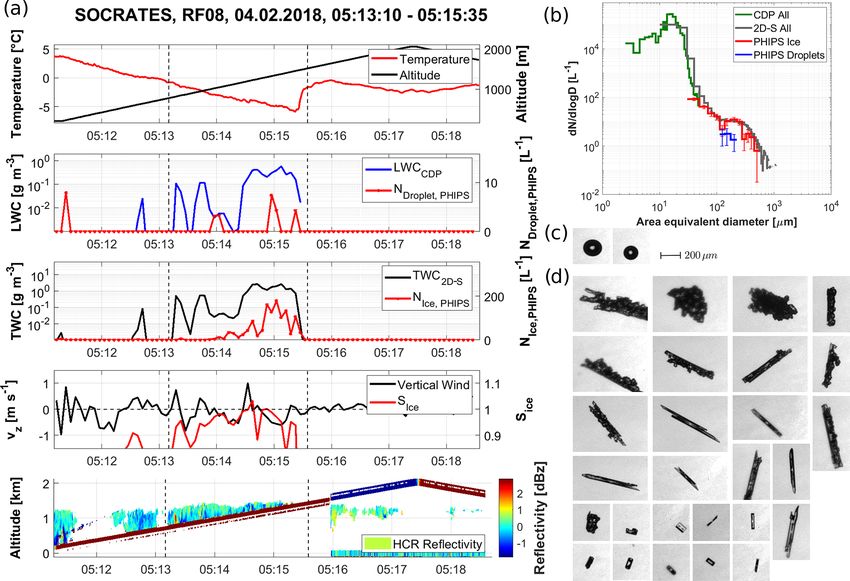
3050            F. Waitz et al.: PHIPS-HALO: the airborne Particle Habit Imaging and Polar Scattering probe – Part 3

   For very small particles below D ≤ 50 µm, the SID fam-          2    Experimental data sets
ily of instruments like the Small Ice Detector mark 3 (SID-
3, Vochezer et al., 2016) and Particle Phase Discriminator         In this work, we use experimental in situ data gathered during
(PPD, Hirst and Kaye, 1996; Kaye et al., 2008; Vochezer            two airborne field campaigns to develop and test a single-
et al., 2016,; Mahrt et al., 2019) offer reliable phase dis-       particle phase discrimination algorithm for the PHIPS probe.
crimination based on the spatial distribution of the forward       The two data sets refer to the two respective campaigns:
scattered light. The SID family of instruments has the disad-          1. ACLOUD – Arctic CLoud Observations Using airborne
vantage, however, of not measuring the phase of each single               measurements during polar Day of May–June 2017
particle but only for a sub-sample. Therefore, a large sam-               based in Svalbard (Spitsbergen, Norway) and
pling time is required to derive ice concentrations in mixed-
phase clouds that are dominated by droplets. The Cloud and             2. SOCRATES – Southern Ocean Clouds, Radiation,
Aerosol Spectrometer with Polarization (CAS-POL, DMT,                     Aerosol Transport Experimental Study of January–
Longmont, CO, USA, Glen and Brooks, 2013) is an instru-                   February 2018 based in Hobart (Tasmania, Australia).
ment that measures the light scattered by single cloud par-
                                                                   An overview of the meteorological and microphysical con-
ticles and aerosols in a size range of 0.6 µm ≤ D ≤ 50 µm
                                                                   ditions as well as the instrumentation during those cam-
in the forward and backward directions. Based on the po-
                                                                   paigns can be found in Knudsen et al. (2018) and Wendisch
larization ratio of the backscattered light, the sphericity of
                                                                   et al. (2019) for ACLOUD and McFarquhar et al. (2019) for
the cloud particles can be determined (Sassen, 1991; Nich-
                                                                   SOCRATES. The sampling during both campaigns includes
man et al., 2016). However, recent studies have suggested
                                                                   a wide variety of different cloud conditions: warm clouds, su-
that particle phase discrimination of polarization-based mea-
                                                                   percooled liquid clouds, ice clouds and mixed-phase clouds.
surements can misclassify up to 80 % of the ice particles as
                                                                   Clouds were sampled in an altitude range from boundary
droplets in the presence of small, quasi-spherical ice (Järvi-
                                                                   layer clouds below 200 m to mid-level clouds between 4000
nen et al., 2016).
                                                                   and 6000 m. Temperatures ranged from −15 to +5 ◦ C dur-
   Hence, in the size range D ≤ 100 µm, methods for reli-
                                                                   ing ACLOUD and −35 to +5 ◦ C during SOCRATES. The
able particle phase discrimination are still needed. The Par-
                                                                   sampled ice particles covered a range of different particle
ticle Habit Imaging and Polar Scattering probe (PHIPS)
                                                                   shapes and habits (columns; plates; needles; bullet rosettes;
is a unique instrument designed to investigate the micro-
                                                                   dendrites; and irregulars, including rough, rimed and pris-
physical and light-scattering properties of cloud particles.
                                                                   tine particles) as well as sizes. More details can be found in
It produces microscopic stereo images whilst simultane-
                                                                   the Supplement (Sect. S1). The instrumentation on the two
ously measuring the corresponding angular-scattering func-
                                                                   aircraft included cloud particles probes such as the SID-3,
tion from 18 to 170◦ for single particles in a size range from
                                                                   CDP (Cloud Droplet Probe, DMT, Longmont, CO, USA),
50 µm ≤ D ≤ 700 µm and 20 µm ≤ D ≤ 700 µm for droplets
                                                                   CIP and PIP (Precipitation Imaging Probe, DMT, Longmont,
and ice particles, respectively. More information and a de-
                                                                   CO, USA) during ACLOUD and 2D-C, 2D-S and CDP dur-
tailed characterization of the PHIPS setup and instrument
                                                                   ing SOCRATES. Due to the variability of the meteorological
properties can be found in Abdelmonem et al. (2016) and
                                                                   conditions and sampled particles, the data gathered during
Schnaiter et al. (2018).
                                                                   these two campaigns make a suitable and representative data
   In this work, we will present a method to discriminate
                                                                   set to develop the phase discrimination and particle size dis-
the phase of single cloud particles based on their angular-
                                                                   tribution algorithms that are presented in this work.
scattering function. An algorithm was developed using ex-
perimental in situ data from two aircraft campaigns target-
ing mixed-phase clouds. We present a method to use single-         3    Single-particle phase discrimination algorithm
particle angular-light-scattering measurements to produce
size distributions for spherical and aspherical particles sep-     The angular-scattering properties of spherical particles can
arately.                                                           be analytically calculated using the Mie theory. The angular-
   This work is structured in the following: in Sect. 2, the       scattering properties of usually aspherical ice particles, how-
aircraft campaigns of the experimental data sets used in this      ever, are much more complex, which significantly alters their
work are introduced. Next, in Sect. 3 the methodology and          scattering properties compared to spherical particles (Järvi-
calibration of the phase discrimination algorithm are ex-          nen et al., 2018; Schnaiter et al., 2018; Sun and Shine, 1994;
plained. In Sect. 4, the particle sizing will be introduced, and   Um and McFarquhar, 2011). Hence, it is possible to differ-
several methods for shattering correction will be discussed.       entiate between the angular-scattering functions (ASFs) of
Finally, in Sect. 5, the described methods will be used in three   spherical and aspherical particles by looking into differences
case studies. The results will be compared to measurements         in the angular-light-scattering behavior in the angular regions
by other cloud particle probes during the same campaigns.          where spherical particles exhibit unique features, like the
                                                                   minimum around 90◦ and the rainbow around 140◦ . In this
                                                                   section, we introduce four scattering features and develop an

Atmos. Meas. Tech., 14, 3049–3070, 2021                                             https://doi.org/10.5194/amt-14-3049-2021
F. Waitz et al.: PHIPS-HALO: the airborne Particle Habit Imaging and Polar Scattering probe – Part 3                                     3051

Figure 1. Stereo micrograph of a droplet (a) and a quasi-spherical ice particle (b) taken by the PHIPS probe. In the stereo micrograph, the
two views of the particle have an angular distance of 120◦ . The instrument concurrently recorded the angular-light-scattering functions of the
imaged particles as displayed in (c). The theoretical scattering function calculated for a droplet with a diameter of 200 µm calculated using
the Mie theory is shown for comparison in (c). The calculated scattering intensity is integrated over the field of view of each of PHIPS’ 20
polar nephelometer channels so it can be compared to the measurement (see Supplement Sect. S6 for details).

                                                                          step, ASFs calculated by the Mie theory (BHMIE, Bohren
                                                                          and Huffmann, 2007) for spherical particles using the refrac-
                                                                          tive index for water (nrefr = 1.332) are compared to modeled
                                                                          ASFs of aspherical ice crystals (Baum et al., 2011 and Yang
                                                                          et al., 2013). Based on the differences in the ASFs, typical
                                                                          features are determined that are characteristic for spherical
                                                                          or aspherical particles (see Fig. 2). The algorithm is then cal-
                                                                          ibrated and validated using PHIPS data from the two field
                                                                          campaigns that were introduced in the previous section. This
                                                                          data set consists of about 23 000 representative single cloud
                                                                          particles of various phases, habits and sizes for which stereo
                                                                          micrographs as well as the corresponding ASFs are available.
                                                                          Those particles are manually classified as spherical or as-
                                                                          pherical based on their appearance in the stereo micrographs.
                                                                          The calibration of the phase discrimination algorithm is then
                                                                          based on the ACLOUD data set only. This way, a classifica-
                                                                          tion probability for every feature is determined. The differ-
                                                                          ent features are then weighed and combined to a final dis-
Figure 2. Visualization of the four classification features: f1 is
the Mie comparison (shaded area between curves and Mie calcu-             crimination probability for every single particle. Lastly, the
lation); f2 is the downslope; f3 is the upslope before the rainbow        data from the SOCRATES campaign are used to validate the
feature; and f4 is the ratio around the minimum at 90◦ . The green        discrimination algorithm and to determine the discrimination
line shows the calculated ASF for a theoretical spherical particle.       accuracy.
The blue area and lines show the measured ASFs of an exemplary
droplet (D = 119.6 µm) and ice crystal (D = 165.8 µm) from the            3.1     Discrimination features
SOCRATES campaign.
                                                                          3.1.1    f1 : comparison with Mie scattering

                                                                          One approach to discriminate between spherical and aspher-
algorithm that is able to classify each particle based on the             ical particles is to compare a particle’s ASF with theoretical
combined information from multiple features of the ASFs                   Mie calculations. To estimate the deviation of the observed
(see Fig. 2).                                                             ASFs from the calculated Mie scattering, we evaluate the
   The basic concept of the development procedure for the                 integrated difference between measurement and calculation
single-particle phase discrimination algorithm will be ex-                (shaded area between the curves in Fig. 2). Figure 4 shows
plained in this section and is shown in Fig. 3. In the first              a step-by-step explanation of the determination of the f1 pa-

https://doi.org/10.5194/amt-14-3049-2021                                                     Atmos. Meas. Tech., 14, 3049–3070, 2021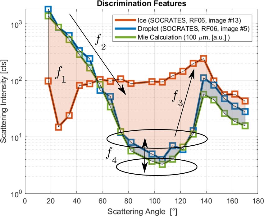
3052 F. Waitz et al.: PHIPS-HALO: the airborne Particle Habit Imaging and Polar Scattering probe – Part 3
Figure 3. Schematics showing the basic working principle of the phase discrimination algorithm.
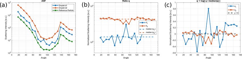
rameter based on two exemplary droplets: a droplet (d1) with To demonstrate that this feature is representing a distinc-
D = 119.6 µm (the same particle as used in Fig. 2) and a the- tive difference between spherical and aspherical particles,
oretical Mie sphere (d2) with D = 200 µm. Figure 4a shows the distribution of the feature parameter value f1 of repre-
the ASFs for the two particles as well as the ASF of the ref- sentative, manually classified spherical and aspherical parti-
erence Mie sphere with D = 100 µm. cles from the experimental in situ aircraft measurement cam-
We define the ratio between the measured intensity Iexp paigns introduced in Sect. 3.3 are shown in Fig. 6a. It can
of an individual particle and the Mie calculation IMie for a be seen that, roughly, if a given particle has a feature value
spherical reference particle with a diameter of 100 µm for of, e.g., f1 < 4.5, it is likely spherical; if f1 > 5, it has a
every nephelometer angle θi of high probability of being an aspherical particle. Phase dis-
crimination based on this feature alone would already allow
Iexp (θi )
q(θi ) = (1) for a reasonable discrimination, but there also exist spheri-
IMie (θi ) cal particles with, e.g., f1 > 5 that would be misclassified by
as shown in Fig. 4b. To be comparable to the measured inten- using this approach. Hence, multiple features are taken into
sities, the calculated theoretical Mie scattering function was account to increase the discrimination accuracy.
integrated over the field of view of the polar nephelometer
channels (see Sect. S6). Ideally, this ratio qi should be cal- 3.1.2 f2 + f3 : down- and upslope
culated with a theoretical reference particle with the same
diameter as the detected particle. However, the diameter of When looking at Fig. 2, the most distinctive differences be-
the measured particle is not known without applying a size tween the ASFs of spherical and aspherical particles are
calibration first. To circumvent this, each qi is normalized the minimum around 90◦ and the rainbow maximum around
by the median over all channels q (dashed line in Fig. 4b). 140◦ for spherical particles, whereas aspherical particles of-
For a spherical particle, this ratio should be approximately ten show a flatter angular-scattering behavior. One way to
q ' const. (see Sect. S2). Since we do not know the diame- extract those features is to evaluate the “exponential slope”
ter of the measured particle without applying a size calibra- of
tion, q is normalized by the median over all channels q, and log(I (θ2 )) − log(I (θ1 ))
the influence of the approximately constant factor can be ne- f2 = (3)
θ2 − θ1
glected. This also has the advantage that we do not need to
calibrate the conversion factor from counts to power unit (W ) in the region before and after the minimum around 90◦ . This
of the photomultiplier array, which can change for different results in two features: the negative slope before the mini-
campaigns, gain settings and changes in laser power. Thus, mum and the positive slope between minimum and rainbow
the discrimination algorithm works for different campaigns around 140◦ . In general, steeper slopes mean that a given
and settings without further calibration. particle is likely to be spherical. The first “slope feature”
Furthermore, as the deviation in “both directions” from the (f2 ) is the “downslope”, which is simply the linear slope
calculated Mie intensity has to be weighted equally, qi = 2 from θ1 = 42◦ to θ2 = 74◦ . The first three scattering chan-
and qi = 12 should be equivalent. Therefore, we make the nels (θ = 18, 26, 34◦ ) are not taken into account here because
transformation qi0 → log(qi /q). The resulting “feature pa- they have a larger possibility of being saturated for larger par-
rameter” is then finally defined as the logarithm of the in- ticles. The slopes are determined by applying a linear fit to
tegral over all angles θi : the logarithmic intensities in the channels between θ1 and θ2 .
Z Z
qi
The second slope feature (f3 ), the “upslope”, is calculated
f1 = log |qi0 | dθi = log log dθi , (2) as the (logarithmic) slope from the minimum around 90◦ to
q
the maximum of the rainbow peak. Since the scattering in-
which corresponds to the area under the curves in Fig. 4c. tensity can be very low and, therefore, comparable to the
Atmos. Meas. Tech., 14, 3049–3070, 2021 https://doi.org/10.5194/amt-14-3049-2021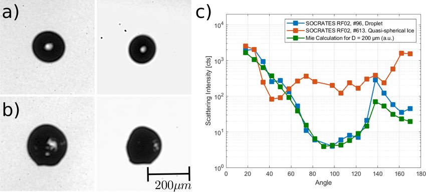
F. Waitz et al.: PHIPS-HALO: the airborne Particle Habit Imaging and Polar Scattering probe – Part 3                                       3053

Figure 4. Determination of the feature parameter f1 of two exemplary droplets: droplet d1 (blue) is the same particle as used in Fig. 2.
Droplet d2 (red) is a theoretical Mie sphere with d = 200 µm. The plots show the particles’ ASFs (a), q and q (b) and q 0 (c). The resulting
f1 is then calculated as the integral over all channels (i.e., area between each curve and y = 0). The resulting values are f1 = 3.7 for d1 and
f1 = 2.2 for d2.

magnitude of the background noise (especially for small par-                     only one channel to minimize the impact of noise. This al-
ticles), the “lower end” is averaged over multiple channels                      lows for the discrimination algorithm to be used for multiple
from θ = 74 to 106◦ . The upper end of the slope is not fixed                    campaigns (even with differing settings or minor hardware
either but rather chosen dynamically, as the angular position                    changes or malfunction) without additional calibration (see
of the rainbow peak can vary within four scattering channels                     Sect. 3.4).
between θ = 130 and 154◦ . Thus, we define the slope fea-
ture f3 as                                                                       3.2   Simulation of the feature parameters

f3                                                                               To prove that the defined set of discrimination fea-
     log (max[I (130 to   154◦ )]) − log (mean[I (74   to   106◦ )])             tures reliably discriminates between spherical and aspher-
=                                                                      ,   (4)   ical particles, we calculate the feature parameter values
                               θ2 − θ1
                                                                                 fi based on theoretical ASFs. For droplets, we use the
with the corresponding angle of the rainbow maximum θ2                           Mie theory for spherical particles with diameters from
and the minimum θ1 = 90◦ . This way, even small particles                        100 µm ≤ D ≤ 700 µm. For ice, we use modeled orientation-
and elongated particles with a shifted rainbow peak (see                         averaged ASFs of ice crystals of different habits and rough-
Sect. S4) can be classified correctly.                                           ness using the databases from Baum et al. (2011) and Yang
                                                                                 et al. (2013) in the size range from 20 µm ≤ D ≤ 700 µm.
3.1.3     f4 : ratio around the 90◦ minimum
                                                                                 Similarly as explained beforehand, the scattering intensities
Another possible way to depict the depth of the 90◦ minimum                      are integrated over the field of view of the polar nephelome-
is to directly compare the intensities in the vicinity around                    ter channels. The distribution of feature parameters is shown
θ = 90◦ with channels that are farther away (see Fig. 2).                        in Fig. 5. It can be seen that the resulting values differ sig-
Hence, the “mid-ratio” feature is defined as                                     nificantly for droplets and ice. This shows that the afore-
                                                                                 mentioned features are in fact fit to discriminate the ASFs
             mean[I (58, 66, 114, 122◦ )]

                                                                                 of spherical and aspherical particles. From now on, we will
f4 = log                                      .            (5)
            mean[I (74, 82, 90, 98, 106◦ )]                                      assume that particles that appear spherical in terms of their
                                                                                 angular-light-scattering behavior are droplets and particles
   With the distinct shape of the ASFs of droplets around                        that appear aspherical in their ASFs are ice. Note that this in-
the 90◦ minimum one could argue that an intensity threshold                      cludes also deformed droplets (as discussed in the Sect. S4)
might be enough to discriminate between spherical and as-                        as well as quasi-spherical ice as shown in Fig. 1.
pherical particles (e.g., classifying every particle with I (θ =
90◦ ) smaller than a certain threshold Ithresh as spherical).                    3.3   Calibration
However, looking at absolute values would prove impracti-
cal, as the ASF scales with particle size: a very small as-                      Next, the discrimination features were applied to experimen-
pherical particle could still fulfill I (θ = 90◦ ) < Ithresh as well             tal data sets of real cloud particles. We used in situ data of
as a rather large spherical particle I (θ = 90◦ ) > Ithresh , re-                representative, manually classified single particles to validate
spectively. Hence, the discrimination features presented here                    the calculated features. These experimental data were then
are all based on relative values, slopes and ratios instead of                   used to calibrate the algorithm (i.e., the classification proba-
discrete thresholds. Further, all discrimination features are                    bility functions Pi (fi ) for every feature), in order to have a
based on the scattering signal of multiple channels instead of                   numerical function that calculates a classification probabil-

https://doi.org/10.5194/amt-14-3049-2021                                                           Atmos. Meas. Tech., 14, 3049–3070, 2021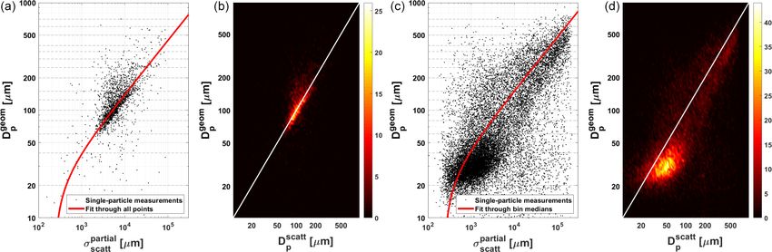
3054              F. Waitz et al.: PHIPS-HALO: the airborne Particle Habit Imaging and Polar Scattering probe – Part 3

Figure 5. Normalized histograms of the discrimination features fi evaluated for theoretical ASFs. Simulated ASFs were calculated using the
Mie theory in the case of droplets (blue) and by selecting typical ice particle habits (red) from the light-scattering databases by Baum et al.
(2011) and Yang et al. (2013). Normal distribution fits to the data are depicted by solid lines in the graphs. Note that the simulations provide
orientation-averaged ASFs, whereas the observed particles by PHIPS have random but fixed orientations.

ity for every feature of a given particle and later a combined            were taken into account, whereas images that show multi-
probability that can be used to discriminate every single par-            ple particles and particles that are only partly imaged, out
ticle based on its phase.                                                 of focus or not clearly distinguishable were ignored. Hence,
   The experimental data sets used for the calibration and                the resulting data set used for the calibration (based on the
verification of the discrimination algorithm are described in             ACLOUD campaign) includes 1853 droplets and 7885 ice
detail in Sect. 2. As it is the goal to develop an algorithm              crystals. The data set used for the validation and determina-
that is suitable without any further calibration for upcom-               tion of the discrimination accuracy (see Sect. 3.4) contains
ing campaigns, the calibration and verification data sets are             2284 droplets and 9936 ice crystals from the SOCRATES
entirely disjunct: the ACLOUD data set is used for calibra-               campaign. The chosen data sets consist of representative
tion; the verification is done using the SOCRATES data set.               cloud particles which cover a wide range of different particle
The ACLOUD and SOCRATES campaigns comprise 14 and                         shapes and habits (columns; plates; needles; bullet rosettes;
15 research flights, during which, in total about 41 000 and              dendrites; and irregulars, including rough, rimed and pris-
235 000 single particles were detected by PHIPS, respec-                  tine particles) as well as sizes D = 20–700 µm and D = 100–
tively. More details about sizes and habits of the manually               700 µm for ice and droplets, respectively.
classified particles used for the calibration can be found in                The left panels of Fig. 6 show, similar to the simulations in
the Supplement (Sect. S1). Because the imaging component                  Fig. 5, the relative amount n(fi ) of particles that share a cer-
of PHIPS has a limited temporal resolution, this results in               tain feature parameter value X. To account for the different
about 22 000 and 32 000 events with matching stereo mi-                   amount of ice and droplets in the data set (Nice ≈ 3·Ndroplet ),
crographs for the ACLOUD and SOCRATES flights, respec-                    the number frequencies ndroplet/ice are normalized by the to-
tively. Based on these stereo micrographs, all imaged parti-              tal amount of droplets and ice particles. The plots show that
cles were manually classified as ice or droplets. To ensure a             the distribution of the four aforementioned feature parame-
representative data set, only clearly distinguishable particles           ters are clearly distinct for droplets and ice and thus repre-

Atmos. Meas. Tech., 14, 3049–3070, 2021                                                      https://doi.org/10.5194/amt-14-3049-2021
F. Waitz et al.: PHIPS-HALO: the airborne Particle Habit Imaging and Polar Scattering probe – Part 3                                        3055

Figure 6. Left: normalized histograms of the discrimination features, f1 , f2 , f3 and f4 , of all manually classified particles (blue: droplets,
red: ice) from the ACLOUD campaign that were used for the calibration of the discrimination algorithm. The histograms can be nicely fitted
by normal distributions (solid lines). Right: corresponding probability for a given particle with a given feature parameter value to be classified
as ice or a droplet, including sigmoidal fits.

sent features that can be used to discriminate droplets from               tributions agree very well. The only exception to this is the
ice. Further, it can be seen that these normalized occurrences             mean value of the distribution of droplets for f1 , which is
n(fi ) are normally distributed. The distributions of the four             shifted slightly to larger values compared to the simulations.
feature parameters based on the measurements (Fig. 6) show                 This is to be expected because the “Mie comparison feature”
a similar trend to the simulations (Fig. 5). The width of the              f1 is based on the relative difference between the measured
distributions of feature parameters for measurements is much               and calculated ASFs. This difference is much smaller for
broader compared to the simulations. This can be explained                 simulated particles as discussed in Sect. 3.1.1.
by the single orientation of the measured crystals compared                   However, Fig. 6 also shows that the ice and droplets modes
to the orientation averaging that was used in the simula-                  are not always clearly separable for every feature and for ev-
tions. Orientation averaging tends to smooth out features in               ery particle. Therefore, instead of using a sharp threshold, a
the ASFs and thus cause more narrow feature parameters. It                 classification probability of
should be also noted that the theoretical computations are for
idealized crystals. Nevertheless, the mean values of the dis-                                    nice (fi )
                                                                           Pi (fi ) =                               ,                         (6)
                                                                                        nice (fi ) + ndroplet (fi )

https://doi.org/10.5194/amt-14-3049-2021                                                         Atmos. Meas. Tech., 14, 3049–3070, 2021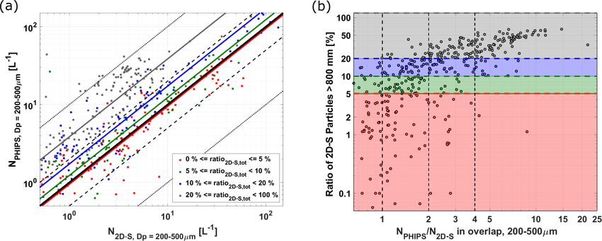
3056             F. Waitz et al.: PHIPS-HALO: the airborne Particle Habit Imaging and Polar Scattering probe – Part 3

where a particle is classified as ice (or with 1 − Pi (fi ) as a     same parameterization still works well for the SOCRATES
droplet) based on the ratio between ndroplet (fi ) and nice (fi )    data set.
for each feature (see right panels of Fig. 6), is defined. As-
suming that ni (fi ) follows normal distributions with com-          3.5   Phase discrimination using machine learning
parable widths, Pi (fi ) can be approximated and fitted by a
sigmoid function. Following that, the probability functions          Binary classification problems like the one presented in this
Pi (fi ) are determined by using a sigmoidal fit for every fea-      work are typically well fit to be solved using machine learn-
ture based on the empiric data. These probabilities, Pi , for        ing (ML) algorithms (Kumari and Srivastava, 2017). For ex-
each feature are combined to                                         ample, in recent works, Mahrt et al. (2019) and Touloupas
                                                                     et al. (2020) have presented different methods to employ
                 n
              1X                                                     ML to discriminate ice and liquid cloud particles using
Pcombined =         wi · Pi (fi )                             (7)
              n i=1                                                  the PPD-HS (High-speed Particle Phase Discriminator) and
                                                                     HOLIMO (HOLographic Imager for Microscopic Objects),
with empiric weights wi that are determined using recursive,         respectively. Depending on the chosen classification prob-
linear optimization. Coincidentally, the optimum weight is to        lem, ML algorithms can be very easy and quick to set up:
weigh all four features equally, i.e., w1 = w2 = w3 = w4 = 1         basically all one needs is a (pre-classified) training data set.
and thus Pcombined = mean(Pi ). Finally, this results in a clas-     There exists software, such as, e.g., TensorFlow (Google
sification probability for every given particle with a set of        LLC, CA, USA), that is specialized on ML; however, nowa-
calculated feature parameter values [f1 , f2 , f3 , f4 ], which is   days most common analysis software such as, e.g., MATLAB
then classified based on Pcombined as a droplet (P ≤ 50 %) or        or Mathematica has built-in ML toolboxes that make work-
ice particle (P > 50 %). Details on the fit parameters for Pi        ing with ML quite easy, fast and comfortable. In general, the
can be found in Appendix A and Appendix B.                           main idea is basically that the ML algorithm is able to iden-
                                                                     tify systematic differences and common features of the dif-
3.4    Discrimination accuracy                                       ferent “types” on its own (even such that could be hard to find
                                                                     for humans) and divide the data set accordingly. This way,
Discrimination algorithms often run in danger of “overtrain-         the ML can classify even new, unknown data sets that “it has
ing” or creating a “lookup table”, resulting in seemingly very       never seen” before. Given a large enough training data set,
good discrimination accuracies that, in reality, are just recre-     ML algorithms can achieve high discrimination accuracies.
ating the “training data” used for calibrating the system but           For comparison with the analytical approach used in this
fail to classify new, “unknown” data sets. In order to avoid         work, the classified data set was analyzed using two differ-
this, the “training” and “test” data set are not only disjunct       ent, basic supervised ML methods, using (a) fine decision
but also from entirely different field campaigns. Furthermore,       tree and (b) linear support-vector machine (SVM). This was
this proves that the algorithm is able to function indepen-          done once for the raw data, i.e., just the scattering intensity of
dently for different campaigns without further calibration.          the 18 scattering channels (the θ = 34 and θ = 90◦ were re-
   The confusion matrices (Fawcett, 2006) for the discrimi-          moved) as well as using the four features [f1 , f2 , f3 , f4 ] pre-
nation algorithm for the two campaigns are shown in Fig. 7.          sented in this work and using both raw intensity and derived
For the SOCRATES data set, 99.7 % of ice particles could             features. Again, the data were trained using the ACLOUD
be correctly classified as ice, and only 29 out of 9936 were         data set and tested against the SOCRATES data set. All par-
misclassified as droplets; 95.8 % of droplets were classified        ticles that had any missing values were discarded. The corre-
correctly, and 95 out of 2284 were misclassified as ice. In          sponding discrimination accuracies are shown in Table 1. It
total, out of all particles, 99.0 % were classified correctly.       can be seen that the different ML methods already show good
Respectively, if a particle is classified as ice (droplet) by the    results. Also, it shows once more that the presented features
algorithm, the expected error (i.e., the probability that the ini-   [f1 , f2 , f3 , f4 ] are indeed fit to represent the difference in
tial particle was actually a droplet) amounts to 0.9 % (1.3 %).      the ASFs. With more fine tuning, especially the discrimina-
Also, 100 % of the theoretical particles used in Sect. 3.2           tion accuracy of the SVM approach might reach the 99 % of
(which were not used for the calibration) were classified cor-       the analytical approach.
rectly. More details about the discrimination accuracy and              However, despite the discussed advantages, ML also has
misclassified particles can be found in the Supplement.              one main disadvantage: it is hard to understand what the al-
   Note that during ACLOUD, one channel (θ = 34◦ ) was               gorithm is doing in detail. Basically, what you end up with
malfunctioning and is hence excluded from the analysis. Dur-         is a black box that classifies input data with a given confi-
ing SOCRATES, the θ = 90◦ channel was observed to be af-             dence, but you cannot tell why. Hence, it is very hard to an-
fected by the background noise in the case of droplets and           alyze which features are relevant for the classification. Fur-
was thus excluded. However, due to the design of the dis-            ther, since the ML knows only statistics, not physics, it is
crimination features (i.e., averaging over multiple channels)        possible that the ML algorithm links the classification to
the implications on the discrimination are reduced, and the          “un-physical parameters” that can introduce systematical bi-

Atmos. Meas. Tech., 14, 3049–3070, 2021                                                https://doi.org/10.5194/amt-14-3049-2021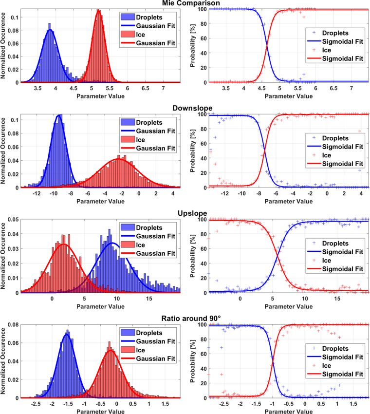
F. Waitz et al.: PHIPS-HALO: the airborne Particle Habit Imaging and Polar Scattering probe – Part 3                                   3057

Figure 7. Confusion matrices that visualize the classification accuracy of the ice discrimination algorithm. The discrimination algorithm was
applied to all manually classified particles from both the ACLOUD (a) and SOCRATES (b) data sets. In both cases the combined probability
Pcombined from the ACLOUD calibration was used to calculate the classification probability of each individual particle.

Table 1. Classification accuracies for different ML approaches and       theless, the presented analytical method works similar to the
different input information.                                             ML approach.

          Used data set       Fine decision    Linear
                              tree             SVM                       4   Particle size distribution
          Raw ASF data        96.4 %           94.4 %                    Since only a sub-sample of the PHIPS particle events pro-
          Derived features    97.9 %           98.4 %                    duce a stereo micrograph (i.e., maximum imaging rate of
          Both                97.6 %           98.4 %
                                                                         3 Hz in ACLOUD and SOCRATES), particle size distribu-
                                                                         tions that are based on the analysis of the images can only
                                                                         be calculated with a limited statistics. Furthermore, particle
                                                                         sizing might be biased for particles with sizes smaller than
ases. For example, it could be possible that the ML algorithm            30 µm, due to the limited optical resolution of the PHIPS
learns that large particles (with a corresponding high total             imaging system (Schnaiter et al., 2018). Hence, in the fol-
scattering intensity) are typically ice, whereas droplets are            lowing section, particle sizing based on the single-particle
typically smaller and hence scatter less light. Thus, it would           ASFs is introduced. The calibration based on the stereo mi-
look at the “amplitude” rather than the “shape” of the ASFs              crographs is done following a similar approach as the phase
and classify all “large particles” as ice. Since the number of           discrimination in the previous section.
large droplets in the used data set is rather small, the overall            In order to calculate a particle number size distribution
discrimination accuracy would be quite high; however there               (PSD) per volume from the single-particle sizing data, as
would be the systematical bias that the few large droplets               shown in Fig. 9, the volume sampling rate of the instrument
would tend to be misclassified.                                          has to be known. This sampling rate is simply the product be-
   Hence and because it yields better discrimination accu-               tween the speed of the aircraft and the sensitive area Asens of
racy, for this work, it was chosen to go with the “analytical            the trigger optics. The size of the sensitive area Asens is deter-
approach” instead of ML. Also, the presented method has the              mined using optical-engineering software. This is presented
advantage, as discussed previously, that it works without cal-           in Sect. 4.2.
ibration for further campaigns, even when single-scattering
channels are malfunctioning (such as, e.g., the θ = 34◦ chan-
nel during ACLOUD) or the laser power is changed (since it
takes only the shape, not the amplitude, into account). Never-

https://doi.org/10.5194/amt-14-3049-2021                                                    Atmos. Meas. Tech., 14, 3049–3070, 2021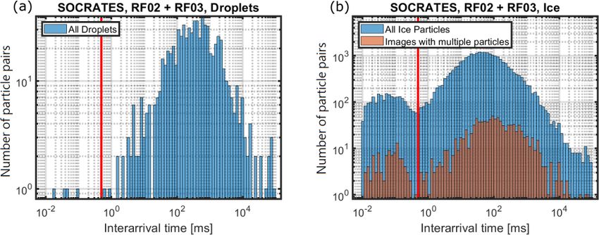
3058                 F. Waitz et al.: PHIPS-HALO: the airborne Particle Habit Imaging and Polar Scattering probe – Part 3

                                                                                                                                         partial
Figure 8. Calibration of the PHIPS-integrated light-scattering intensity measurement, expressed by the partial scattering cross section σscatt ,
                                 geom
against the geometric diameter Dp       deduced from the concurrent stereo micrographs. Stereo micrographs from the SOCRATES data set
were manually classified for droplets (a, b) and ice particles (c, d).

4.1       Particle sizing                                                 and cBG is the integrated background intensity. As already
                                                                          discussed in the previous section, ice and droplets have
The individual detector channels of the PHIPS nephelome-                  vastly differing angular-scattering characteristics, i.e., scat-
ter measure scattered-light intensity I (θ ) of individual cloud                                  diff (θ ). Hence, different a coefficients
                                                                          tering cross sections σscatt
particles that can be converted to a differential scattering              are needed, and the calibration is done separately for ice and
                diff (θ ) as
cross section σscatt                                                      droplets. The coefficient a is calibrated based on the geo-
                                                                                                                         geom
 diff                            2                                        metric cross-section equivalent diameter Dp          derived from
σscatt (θ ) = I (θ )/Iinc · π · dlaser /4,                       (8)      the stereo micrographs. A correction for the slight size over-
with Iinc and dlaser being the power and diameter of the inci-            estimation of the CTA 2 (camera telescope assembly) for
dent laser beam, respectively. Note that I (θ ) in Eq. (8) has            small particles due to the lower magnification is applied (see
to be corrected for possible background intensity due to stray            Schnaiter et al., 2018). More details on PHIPS image analy-
light in the instrument as well as dark photon counts of the              sis routines can be found in Schön et al. (2011).
photomultiplier array. Integrating Eq. (8) over all nephelome-               Similar to the calibration of the phase discrimination al-
                                                       partial            gorithm, manually classified imaged particles were used as
ter channels gives a partial scattering cross section σscatt of
                                                                          a calibration data set. The data are binned with respect to
the particle as defined for the PHIPS measurement geometry
                                                                          the particle’s geometrical area equivalent diameter. The bin
of
                                  Z                                       edges are the same as used for the final PSD data product.
  partial       2                                                         Those are 20, 40, 60, 80, 100, 125, 150, 200, 250, 300, 350,
σscatt = π · dlaser /(4 · Iinc ) · I (θ ) dθ.                 (9)
                                                                          400, 500, 600 and 700 µm. For ice, the coefficient a is de-
                                                                          termined by fitting Eq. (10) through the median of each bin.
                               partial
For spherical particles, σscatt is approximately proportional             For droplets, the function is fitted through all data points,
to their geometrical cross section π · Dp2 /4, with Dp the par-           since the data points are distributed over fewer size bins.
ticle diameter. This is demonstrated in the Supplement using              The background intensity cBG is determined as the integrated
Mie calculations (Sect. S2). Assuming that this is valid not              intensity from forced triggers averaged over time periods
only for spherical droplets but also for aspherical ice parti-            when no particles were present. cBG is the same for droplets
cles, the scattering cross-section equivalent particle diameter           and ice. The calibration is performed for each campaign
Dpscatt can be deduced from the PHIPS intensity measurement               separately, assuming that the instrument parameters remain
I (θ ) as                                                                 unchanged over the duration of one campaign. The result-
                Z                       1                               ing calibration of the scattering equivalent diameter for the
                                          2
                                                                          SOCRATES campaign is shown in Fig. 8a and b for droplets
Dpscatt   =a·        I (θ ) dθ − cBG          .                 (10)
                                                                          and ice, respectively. The corresponding fit parameters are
                                                                          aice = 1.4167 and adroplet = 1.4441. The background mea-
In Eq. (10), a is a calibration coefficient that describes the            surement value is cBG = 238.12.
incident laser properties, the detection characteristics of the              Using this calibration Fig. 9 shows the comparison of
polar nephelometer (e.g., the photomultiplier gain settings)              the particle size distributions averaged over all flights of
and the angular-light-scattering properties of the particle,

Atmos. Meas. Tech., 14, 3049–3070, 2021                                                      https://doi.org/10.5194/amt-14-3049-2021
F. Waitz et al.: PHIPS-HALO: the airborne Particle Habit Imaging and Polar Scattering probe – Part 3 3059
particle sizes. Moreover, as (aspherical) ice particles usually
have different differential scattering cross sections compared
to (spherical) droplets, especially in side scattering directions
where the trigger optics is located, Asens is expected to be de-
pendent also on the phase of the cloud particles. Therefore,
we simulated the size dependence of Asens for spherical and
aspherical particles separately using the FRED Optical En-
gineering Software (Photon Engineering, LLC, USA), which
combines light propagation by optical raytracing simulations
with three-dimensional computer-aided design (CAD) visu-
alization.
For the FRED simulations, the actual PHIPS trigger op-
tics and three-dimensional laser intensity distribution were
reconstructed in the three-dimensional CAD environment of
the software resulting in the actual intensity field the particle
is exposed to when penetrating the sensitive area of the in-
strument. Particles were step-wise positioned at different x,
Figure 9. Comparison of PSD calculated from ASFs using the cali- y and z position across the trigger field of view and depth of
geom
bration defined in Eq. (10) (dotted line) and PSDs based on Dp
field to get a map of the scattered-light intensity that reaches
derived from stereo micrographs (average of CTA1 and CTA2, solid
the sensitive area of the trigger detector. Similar to the actual
line) for droplets (blue) and ice particles (red). The data are from all
flights recorded during SOCRATES. Only stereo micrographs that measurement, a threshold value for the simulated detector
showed only one completely imaged particle were taken into ac- intensity was used that would trigger the system and, there-
count. The same particles were used for both size distributions. fore, defines Asens . This threshold was deduced by mapping
the sensitive area of the instrument in the laboratory using a
piezo-driven droplet dispenser which generates single 80 µm
diameter water droplets (Schnaiter et al., 2018). Equating
Asens from the laboratory mapping with Asens for the corre-
sponding 80 µm FRED simulation then defined the threshold
value that has to be used for all FRED simulations to calcu-
late the size dependence Asens .
The FRED simulations were performed for spherical par-
ticles with the refractive index of supercooled liquid water
(n = 1.3362 + i1.82 × 10−9 ) and the three sizes of 80, 300
and 600 µm. The resulting Asens are shown in Fig. 10 in grey
color. Additionally, to validate the method, Asens was also
estimated using the Mie theory to calculate the differential
scattering cross section for the trigger direction and multi-
ply the results with the actual intensity field as defined by
the FRED simulations. Although Mie calculations are faster
to conduct, these calculations have the disadvantage that they
Figure 10. Sensitive area based on FRED simulations for ice (red) assume a dimensionless particle, which induces uncertainties
and droplets (grey). at the boundaries of the trigger field of view. Yet, the FRED
simulations compare reasonably well with the results of the
Mie calculations.
SOCRATES for both ice (red) and droplets (blue). It can Ice particles were simulated roughened spheres whose sur-
be seen that the size distribution based on the images (solid face light scattering was defined by the ABg model (Pfisterer,
lines) agrees well with the size distribution based on the 2011). A refractive index of n = 1.3118+i2.54×10−9 (War-
angular-light-scattering functions (dotted lines). ren, 1984) was used for the ice simulations. The roughened
ice sphere approach was chosen here to avoid computation-
4.2 Sensitive area ally expensive orientation averaging, which was necessary in
the case of using a non-spherical particle habit. The FRED
Due to the fact that the scattering laser of PHIPS has Gaus- simulations for ice particles were conducted for the five par-
sian intensity profiles and the field of view of the trigger op- ticle sizes of 80, 150, 300, 450 and 600 µm. As can be seen in
tics shows gradual detection boundaries, Asens is expected Fig. 10, the Asens values for ice are significantly larger than
to be size dependent with a larger sensing area for larger those for water droplets of the same diameter. An exponen-
https://doi.org/10.5194/amt-14-3049-2021 Atmos. Meas. Tech., 14, 3049–3070, 20213060 F. Waitz et al.: PHIPS-HALO: the airborne Particle Habit Imaging and Polar Scattering probe – Part 3
Figure 11. Histogram of interarrival times of ice particles (a) and droplets (b) measured during SOCRATES flights RF02 and RF03. Com-
parison of the interarrival times of all particles (blue) and only particles whose images were manually classified as shattering events (red).
The red vertical line marks the τ ≤ 0.5 ms threshold.
tial function was fitted to the FRED results to get Asens as whether or not a cloud segment was affected by shattering in
a function of particle diameter. These functional dependen- individual cases.
cies are then used to calculate the volume sampling rate that
is required to convert the single-particle data to particle size 4.3.1 Interarrival time analysis
distributions.
The most common method to detect shattering is based on
4.3 Correction for shattering artifacts the analysis of particle interarrival times (Field et al., 2003).
If two (or more) particles are detected in very short succes-
One major source of uncertainty for wing-mounted probes is sion, those particles are identified as shattering fragments and
the shattering of ice particles on the instrument’s outer me- removed. Figure 11 shows a histogram of interarrival times
chanical structures or breakup of particles in the instrument (τ ) of ice particles (left) and droplets (right) measured dur-
inlet. An example of the shattering of a large particle and ing two flights of SOCRATES. For ice, it is apparent that the
breaking up of aggregates in the inlet flow field can be found otherwise approximately log-normal distributed interarrival
in the Supplement (Sect. S5). Shattering can lead to a signif- times show a second, lower mode below τ ≤ 0.5 ms (equiva-
icant overcounting of ice particles (e.g., up to a factor of 5 lent to spatial separation of ≤ 7.5 cm, assuming a relative air
using a fast forward scattering spectrometer probe (FSSP), speed of v = 150 m s−1 ) that is likely caused by shattering.
Field et al., 2003) and a bias in the particle size distribu- For droplets, the second mode is not visible, since droplets
tion towards smaller sizes. Here, we characterized the fre- tend to less fragment when entering the instrument inlet.
quency of shattering events in the SOCRATES data set and Whereas the interarrival time analysis method is used in
present a method to detect shattering events within the PHIPS multiple optical array probes (2D-S and 2D-C, Field et al.,
data sets. Even though the geometry of PHIPS was designed 2003), the application is limited for single-particle instru-
to minimize disturbances and turbulences in the instrument ments, like PHIPS, due to their small sensitive area. Near the
(e.g., sharp edges at the front of the inlet and an expanding detection volume, the inlet has a diameter of 32 mm, whereas
diameter of the flow tube towards the detection volume; see the sensitive area measures only about 0.7 mm (depending on
Abdelmonem et al., 2016), shattering can still be an issue, es- phase and size, as discussed in Sect. 4.2), which means that
pecially in clouds where large cloud particles and aggregates the probability of detecting two (or more) fragments of the
with D > 1 mm are present. same shattering event is very low. Furthermore, the instru-
Since the field of view of the camera telescope assembly ment has a dead time of t = 12 µs after each trigger event
(CTA) is much larger (typically ' 1.5 × 1 mm) compared to (Schnaiter et al., 2018). Shattering fragments that pass dur-
the sensitive trigger area (see previous section), the stereo mi- ing this time are not detected. As shown in Fig. 11, only a
crographs can be used to detect shattering events. However, small percentage of the particles whose images were manu-
as only a subset of detected particles is imaged, a shattering ally classified as shattering (red) could be identified as shat-
correction based on inspection of the stereo micrographs is tering using the interarrival time analysis method. Hence it
not a practical and reliable solution. Still, manual examina- can be concluded that interarrival time analysis alone is not
tion of the stereo micrographs can be helpful to determine able to be a reliable shattering flag, either. Nevertheless, all
Atmos. Meas. Tech., 14, 3049–3070, 2021 https://doi.org/10.5194/amt-14-3049-2021F. Waitz et al.: PHIPS-HALO: the airborne Particle Habit Imaging and Polar Scattering probe – Part 3 3061
Figure 12. (a) Comparison of the total number concentrations of 2D-S and PHIPS. Each point is averaged over 30 s. The color code is based
on the ratio of large 2D-S particles with Dmax ≥ 800 µm. The thick black line marks the 1 : 1 line; the dashed and dotted lines are a factor of 2
and 10. (b) Correlation of the ratio of number concentrations of PHIPS and 2D-S and the presence of large 2D-S particles. The horizontal
line marks the 10 % threshold. The color code is the same as in (a).
particles with a low interarrival time τ ≤ 0.5 ms are removed ing flag to mark cloud segments that are potentially affected
and excluded from the analysis. In the next section, a shatter- by shattering. In segments where the 2D-S did not detect any
ing flag is introduced that flags segments which are affected particles or was not measuring, for any reason, 2D-C data
by particle shattering so they can be excluded from further are used instead. That means cloud segments with more than
analysis. 10 % of large particles are removed for future analysis. For
the SOCRATES data set, 44 % of all 1s segments are flagged
4.3.2 Shattering flag based on the presence of large as shattering. This means that about half of all 30 s segments
particles in mixed-phase clouds and approximately 75 % of purely ice
clouds are removed. Droplet-dominated cloud segments are
It is known that a particle’s shattering probability is strongly not affected by this shattering flag.
size dependent. Large particles and aggregates are much
more prone to shattering compared to small particles. To 4.4 Discussion: particle size distribution and statistical
overcome the limitation of the interarrival time method to significance
eliminate shattered particles, we introduce a shattering flag
based on the presence of large particles. Figure 12a shows The sampled cloud volume Vs per unit time t calculates as
the total number concentration of particles in the size over- Vs = Asens · v · t, where v is the relative air speed and Asens
lap region of PHIPS and 2D-S (200 µm ≤ D ≤ 500 µm) for is the probe’s sensitive area. Asens is dependent on particle
all SOCRATES flights. The data are averaged over 30 s seg- phase and diameter, as discussed in Sect. 4.2. Assuming a
ments. Only segments with N2D-S, overlap ≥ 0.5 L−1 are taken relative air speed of v = 150 m s−1 , the resulting sample vol-
into account. The color code indicates the fraction of 2D-S ume amounts to about Vs = 0.08 (0.026, 0.12) L s−1 for ice
particles in the size range of Dmax ≥ 200 µm that are larger particles with diameter D = 200 (50, 500) µm, respectively.
than 800 µm. The diagonal lines mark the median ratio be- This is somewhat larger compared to other single-particle
tween NPHIPS /N2D-S of each color. Figure 12b shows the cloud instruments (e.g., the CPI, Vs = 0.009 L s−1 ; Lawson
correlation of the difference between PHIPS and 2D-S in the et al., 2001), comparable to, e.g., the SID3 (Vs = 0.071 L s−1 ,
overlap region and the ratio of large particles. It can be seen Vochezer et al., 2016) but is significantly smaller compared
that the two probes agree very well in segments with only a to the optical array probes like the 2D-C (Vs ' 0.1−10 L s−1 ,
few large particles. Wu and McFarquhar, 2016). This has consequences for the
In segments that consist of more than 10 % of large parti- averaging time needed in order to achieve statistically signif-
cles, PHIPS and 2D-S tend to disagree, and PHIPS can over- icant information on total particle concentrations.
estimate particle concentrations up to a factor > 10. This can We investigated the statistical uncertainty in example sit-
be explained by the shattering of large particles on the instru- uations for the total number concentration for the size range
ment inlet tip or wall or disaggregation of large aggregates from 20 to 200 µm. This size range was chosen, since at sizes
due to shear forces in the inlet flow. Therefore, said marker below 200 µm the phase information from PHIPS is of inter-
for the presence of large particles will be used as a shatter- est as phase detection based on traditional imaging methods
https://doi.org/10.5194/amt-14-3049-2021 Atmos. Meas. Tech., 14, 3049–3070, 20213062 F. Waitz et al.: PHIPS-HALO: the airborne Particle Habit Imaging and Polar Scattering probe – Part 3
Table 2. Averaging time that is needed until n = 100 particles are sampled as well as the total number of particles sampled during an averaging
time of 30 s, calculated for the size bin of 20–200 µm and exemplary particle concentrations.
q
Dlower edge Dupper edge Concentration tn=100 nt=30 s n−1
t=30 s
[L−1 ] [s] [%]
20 200 1 1688.5 1.8 75.0
20 200 10 168.9 17.8 23.7
20 200 56.3 30 100 10
20 200 100 16.9 177.7 7.5
20 200 1000 1.7 1776.8 2.4
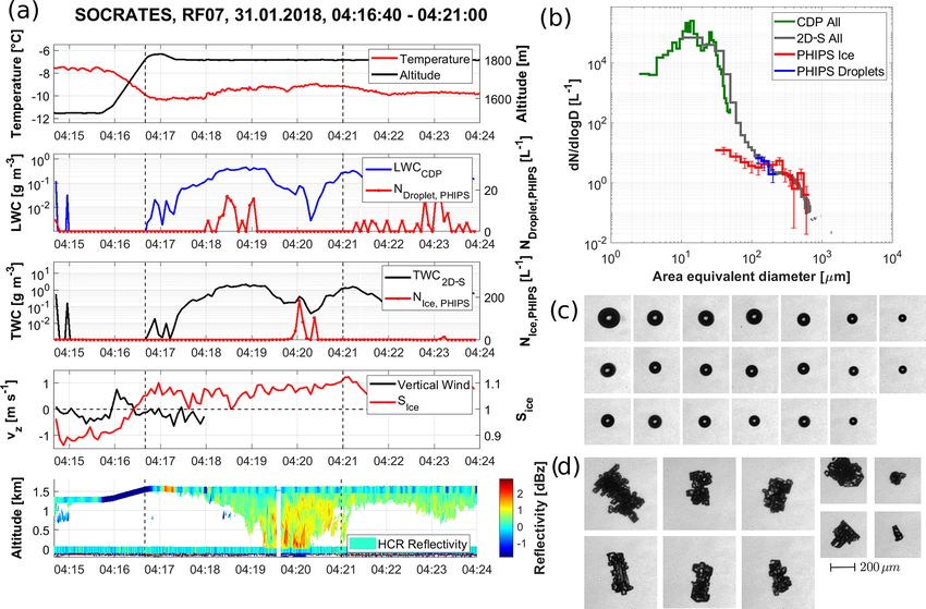
Figure 13. Example of PHIPS data acquired in a low-level supercooled liquid cloud over the Southern Ocean during the SOCRATES
campaign (research flight RF04). (a) Overview of meteorological parameters, CDP, 2D-S and PHIPS number concentrations (based on the
data) as well as HCR radar data. (b) The comparison of the PSDs measured by CDP, 2D-S and PHIPS including statistical uncertainty
ASF √
bars n−1 as discussed in Sect. 4.4. (c) Representative stereo micrographs of particles during that segment measured by PHIPS.
can be challenging for small particle sizes. In order to reach certainty below 10 % within 30 s. For ice crystal concentra-
statistical uncertainty ∝ n−0.5 of less than 10 %, the number tions of 1 (10) L−1 an averaging time of 28 (2.8) min would
of particles per size bin needs to be larger than n > 100. Ta- be needed, which at least in the case of low (< 10 L−1 ) ice
ble 2 shows the calculated averaging time in seconds that is crystal concentrations would likely exceed the sampling du-
needed until n = 100 particles are sampled per bin (tn=100 ) ration. For optical array probes assuming a sampling volume
and the estimated number of particles that would be sampled of Vs = 1.5 L s−1 the corresponding sampling times would
during 30 s of sampling (nt=30 s ), as well as the correspond- be 66.7 s and 6.7 s for concentrations of 1 and 10 L−1 . This
ing −0.5 for a sampling period of 30 s
q statistical uncertainty n shows that in order to get statistically significant size distri-
( n−1 butions, it is important to properly consider adequate aver-
t=30 s ) for the chosen size range. All particles were as-
sumed to be ice. aging time and/or bin size, especially in segments with low
It can be seen that the ice crystal concentrations need to particle concentration.
be larger than 56.3 L−1 in order to achieve a statistical un-
Atmos. Meas. Tech., 14, 3049–3070, 2021 https://doi.org/10.5194/amt-14-3049-2021You can also read