Turbulent diffusion of streaming cosmic rays in compressible, partially ionized plasma
←
→
Page content transcription
If your browser does not render page correctly, please read the page content below
MNRAS 519, 1503–1525 (2023)                                                                                        https://doi.org/10.1093/mnras/stac3207
Advance Access publication 2022 November 9

Turbulent diffusion of streaming cosmic rays in compressible, partially
ionized plasma
Matt L. Sampson ,1 ‹ James R. Beattie ,1 Mark R. Krumholz ,1,2 Roland M. Crocker ,1
Christoph Federrath 1,2 and Amit Seta 1
1 Research   School of Astronomy and Astrophysics, Australian National University, Canberra, ACT 2611, Australia
2 Australian  Research Council Centre of Excellence in All Sky Astrophysics (ASTRO3D), Canberra, ACT 2611, Australia

                                                                                                                                                            Downloaded from https://academic.oup.com/mnras/article/519/1/1503/6815731 by New York University user on 18 January 2023
Accepted 2022 November 3. Received 2022 August 1; in original form 2022 May 18

ABSTRACT
Cosmic rays (CRs) are a dynamically important component of the interstellar medium (ISM) of galaxies. The ∼GeV CRs that
carry most CR energy and pressure are likely confined by self-generated turbulence, leading them to stream along magnetic
field lines at the ion Alfvén speed. However, the consequences of self-confinement for CR propagation on galaxy scales
remain highly uncertain. In this paper, we use a large ensemble of magnetohydrodynamical turbulence simulations to quantify
how the basic parameters describing ISM turbulence – the sonic Mach number, M (plasma compressibility), Alfvén Mach
number, MA0 (strength of the large-scale field with respect to the turbulence), and ionization fraction by mass, χ – affect the
transport of streaming CRs. We show that the large-scale transport of CRs whose small-scale motion consists of streaming
along field lines is well described as a combination of streaming along the mean field and superdiffusion both along (parallel
to) and across (perpendicular to) it; MA0 drives the level of anisotropy between parallel and perpendicular diffusion and χ
modulates the magnitude of the diffusion coefficients, while in our choice of units, M is unimportant except in the sub-Alfvénic
(MA0  0.5) regime. Our finding that superdiffusion is ubiquitous potentially explains the apparent discrepancy between CR
diffusion coefficients inferred from measurements close to individual sources compared to those measured on larger, Galactic
scales. Finally, we present empirical fits for the diffusion coefficients as a function of plasma parameters that may be used as
subgrid recipes for global ISM, galaxy, or cosmological simulations.
Key words: magnetohydrodynamics (MHD) – turbulence – methods: numerical – (ISM:) cosmic rays.

                                                                                of molecules (Cesarsky & Volk 1978; Padovani, Galli & Glassgold
1 I N T RO D U C T I O N
                                                                                2009; Glover et al. 2010; Everett & Zweibel 2011; Drury & Downes
The role that the non-thermal particles known as cosmic rays (CRs)              2012; Grassi et al. 2014; Padovani et al. 2020).
play in both star formation and galaxy evolution is one of the largest             CRs having comparable energy density to other components of
open questions in modern astronomy. Within the diffuse interstellar             the ISM is a necessary but not sufficient condition for them to be
medium (ISM), CRs are important dynamically because their energy                dynamically important. To be dynamically important, sufficiently
densities – directly measured at the Earth and indirectly inferred at           large gradients in CR energy densities must develop; as the transport
larger distances in the Milky Way and in extragalactic systems – are            of CRs largely determines these gradients, it is important to get an
comparable to those in other interstellar reservoirs, such as turbulent         accurate description of the diffusion of CRs.
motions of gas, magnetic fields, interstellar radiation, and self-gravity          Since they are charged, CRs propagate via spiralling around
(Spitzer & Arny 1978; Boulares & Cox 1990; Ferriere 2001; Draine                magnetic field-lines under the Lorentz force. This motion means CRs
2010; Grenier, Black & Strong 2015). As a result, CRs may play an               are coupled to the magnetic fields existing in astrophysical plasmas
important role in either initiating or sustaining galactic winds and            (Strong, Moskalenko & Ptuskin 2007; Grenier, Black & Strong 2015;
in regulating star formation (e.g. Socrates, Davis & Ramirez-Ruiz               Grenier et al. 2015; Gabici et al. 2019), but it also means that CRs
2008; Salem, Bryan & Hummels 2014; Simpson et al. 2016; Pakmor                  can interact resonantly with Alfvén waves whose wavelengths are
et al. 2016; Girichidis et al. 2016; Ruszkowski, Yang & Zweibel 2017;           comparable to their radius of gyration. These resonant interactions
Mao & Ostriker 2018; Hopkins et al. 2021a, b; Crocker, Krumholz &               scatter CRs by altering the pitch angle between the CR velocity
Thompson 2021a, b). In the denser parts of the ISM that are shielded            vector and the local magnetic field. The Alfvén waves responsible
from ultraviolet starlight, CRs play a vital role in determining the            for resonant scattering can either be part of a turbulent cascade
distribution of thermal energy and the ionization state and in initiating       initiated by large-scale disturbances of the ISM (e.g. supernova
many of the chemical reaction chains that give rise to the formation            blast waves), or can be generated by the CRs themselves via the
                                                                                streaming instability (e.g. Kulsrud & Pearce 1969; Wentzel 1974;
                                                                                Farmer & Goldreich 2004; Bell 2013). Low-energy CRs (࣠10–
   E-mail: matt.sampson@princeton.edu                                          100 GeV in Milky-Way-type galaxies and up to ∼10 TeV in

© 2022 The Author(s)
Published by Oxford University Press on behalf of Royal Astronomical Society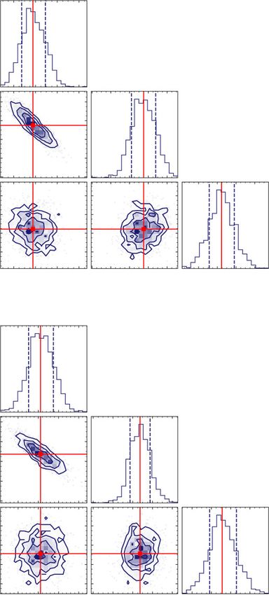
1504        M. L. Sampson et al.
starbursts – Krumholz et al. 2020), which dominate the total CR             been efforts to develop theories for these quantities (Yan & Lazarian
energy budget, are numerous enough and have small enough gyro-              2002, 2004, 2008; Shalchi et al. 2004, 2009; Lazarian & Beresnyak
radii that self-excitation is likely dominant for them. This leads to a     2006; Beresnyak, Yan & Lazarian 2011; Zweibel 2013; Evoli &
situation of self-confinement, whereby CRs stream along magnetic            Yan 2014; Cohet & Marcowith 2016; Shukurov et al. 2017; Zhao
field lines at the same speed as the Alfvén waves they generate in the     et al. 2017; Dundovic et al. 2020; Krumholz et al. 2020; Reichherzer
ionized component of the gas, and in a direction opposite the gradient      et al. 2020, 2022), robust parameter studies probing the relations
in CR pressure.1 In this paper, we will refer to populations of CRs         between the plasma properties and CR diffusion over a wide range of
that have been self-confined to stream along magnetic field lines at        parameter space are lacking. Thus, we still lack a complete effective
roughly the ionic Alfvén speed as streaming cosmic rays (SCRs).            theory of CR transport that can be used in simulations or models
   While streaming may be the correct description of CR transport on        that do not resolve the characteristic scales on which CR transport

                                                                                                                                                     Downloaded from https://academic.oup.com/mnras/article/519/1/1503/6815731 by New York University user on 18 January 2023
scales comparable to CR gyroradii ( 1 pc for ∼GeV CRs), there is           becomes effectively diffusive, and thus a pure streaming description
ample evidence that CR transport can be described approximately as          becomes inadequate.
diffusive when measured on molecular cloud or even galactic scales             This issue is of broad importance for understanding the role of
(e.g. Krumholz et al. 2020). Direct in situ observations of high-           CRs in the ISM. Thus, far attempts to address, it have mostly
energy CRs reaching the Solar system indicate that their directions         proceeded empirically, for example by carrying out simulations
of travel are very close to isotropic, as would be expected for             or making models using a wide range of candidate CR transport
diffusive transport; models based on diffusion have successfully            prescriptions and seeing which ones best match observations (e.g.
reproduced a large number of observations (e.g. Strong et al. 2007;         Gabici et al. 2010; Jóhannesson et al. 2016; Lopez et al. 2018; Chan
Zweibel 2017, and references therein). Nor is it surprising that such       et al. 2019; Crocker et al. 2021b; Hopkins et al. 2021b). However,
a description applies: even if CRs move purely by streaming along           this approach has its limitations: it can determine what parameter
field lines, interstellar plasmas are turbulent (see Federrath 2016, for    values best fit the data within the context of a particular model but
a review), and so the field lines themselves are neither straight nor       cannot tell us if that model is missing essential ingredients. Nor do
time independent. Thus, even if on small scales CRs did not diffuse         these observations, which are largely limited to the Milky Way and
at all, just the turbulent motion of the magnetic field lines to which      its nearest neighbours, provide much insight into how CR transport
they are bound should induce diffusion-like behaviour.                      might differ in more distant galaxies whose interstellar environments
   In principle, it should be possible to compute diffusion coefficients    differ from those found locally (e.g. Krumholz et al. 2020). In this
to describe this process in terms of the parameters that describe the       paper, we therefore attempt a different approach: assuming that
magnetized turbulence, most prominently the sonic Mach number               self-confinement and streaming are the most relevant mechanisms
M, Alfvén Mach number MA , and ionization fraction χ . These               for CR transport on small scales, at least for the low-energy CRs
diffusion coefficients could be quite different from the traditional        that dominate the CR pressure budget, we seek to determine an
spatial diffusion coefficient for CRs that can be computed from, e.g.       effective theory for CR diffusion when measured over larger scales.
quasi-linear theory (QLT), because they describe a very different           We do so over a very wide range of plasma parameters, combining
process, averaged over very different scales. The traditional CR            numerical simulations of magnetohydrodynamic (MHD) turbulence
diffusion coefficient from QLT is fundamentally a result of CRs             with those of CR transport through this turbulence and using the
making random walks in pitch angle, which leads them to perform             results as a series of numerical experiments to which we can fit a
a corresponding random walk in space along the magnetic field.              model.
The characteristic size scale over which it is reasonable to describe          The plan for the remainder of this paper is as follows. We describe
this process as a random walk, and thus as diffusive, is the mean           the set-up of our numerical experiments in Section 2 and show the
distance that CRs travel before resonant scattering off incoherent          results in Section 3. We use these results to build up an effective
Alfvén waves causes their pitch angles to randomize; this is much          theory for CR transport in Section 4 and summarize our findings in
smaller than the characteristic scales associated with interstellar         Section 5.
turbulence. By contrast, the diffusion coefficients associated with
turbulent motion of the gas can only be defined on scales comparable
                                                                            2 METHODS
to the sizes of turbulent eddies in the flow, and the diffusion they
describe does not depend on rates of pitch angle scattering. Indeed,        Our goal is to measure the effective diffusion coefficient for CRs
the turbulent diffusion could be non-zero even if the CR pitch              streaming along field lines in turbulent plasmas, across a wide range
angle distribution were a δ-function, corresponding to no small-            of plasma parameters. To this end, we construct a simulation and
scale diffusion at all. Similarly, even though random walks in pitch        analysis pipeline in several steps. We first perform MHD simulations
angle only induce diffusion along field lines (at least to linear order),   to produce background plasmas through which we can propagate
turbulence can induce diffusion perpendicular to the direction of the       CRs. We discuss the details of the MHD simulations in Section 2.1.
mean field.                                                                 Our second step is to simulate the streaming of CRs through these
   Since most observational constraints on the rate at which CRs            plasmas, a process we describe in Section 2.2. In the final step,
diffuse are sensitive to scales comparable to (or greater than) the         we construct a forward model for the CR position distribution
scales of interstellar turbulence, rather than the much smaller scales      that we can compare to our simulation results to infer large-scale
of CR isotropization, the effective rate of diffusion expected for SCRs     diffusion parameters. We outline this model and our fitting method
at those larger scales is of considerable interest. While there have        in Section 2.3.
                                                                               We apply our pipeline to simulations at a range of sonic Mach
                                                                            number M, Alfvén Mach number MA0 and ionization fraction (by
1 Itshould be made clear here that individual CR particles still move at    mass) χ . The first two of these describe the plasma itself, while χ
velocity ∼ speed of light. However, due to the constant randomization in    affects the speed at which CRs stream, since the streaming speed
pitch angle, the mean position of self confined CR populations propagates   is set by the ion Alfvén speed rather than the total Alfvén speed.
along the magnetic field lines at roughly the ion Alfvén speed.            We alter both M and MA0 in the MHD simulation runs, while χ

MNRAS 519, 1503–1525 (2023)
Cosmic ray diffusion 1505
is an input parameter for the CR propagation simulation step. The dump an MHD realization of the 3D field variables every t = τ /10.
parameter values we sample are M ∈ [2, 4, 6, 8, 10], MA0 ∈ [0.1, For our main results, we discretise the L3 domain into 5763 cells. Both
0.5, 1, 2, 4, 6, 8, 10], and log χ ∈ [−5, −4, −3, −2, −1, 0]. These the grid resolution and the temporal resolution are determined via
values are chosen to capture the diversity of M and MA encountered convergence tests detailed in Appendix A. The choice of resolution
in the ISM (Tofflemire, Burkhart & Lazarian 2011; Burkhart et al. here is made based on the analysis of the CR propagation post-
2014). We carry out runs with every possible combination of these processing results, as opposed to an analysis of parameters of the
parameters, for a total of 240 trials. The naming convention for MHD data set itself.
the trials is MxMAyCz where x is M, y is MA0 (with the decimal
point omitted), and z is equal to −log χ . Thus, for example trial
M2MA05C4 has M = 2, MA0 = 0.5, and χ = 1 × 10⁻⁴ . 2.2 Cosmic ray propagation simulations
Downloaded from https://academic.oup.com/mnras/article/519/1/1503/6815731 by New York University user on 18 January 2023
With the MHD simulations in hand, our next step is to simulate
2.1 MHD simulations the propagation of CRs streaming through them. We envision that
each of our simulation boxes is subject to a large-scale CR pressure
We generate turbulent MHD gas backgrounds through which we can gradient, on scales much larger than the box scale, so that CRs stream
propagate CRs using a modified version of the FLASH code (Fryxell through the simulation box in a single direction. We further assume
et al. 2000; Dubey et al. 2008), utilizing a second-order conservative that our boxes are much larger than the size scale on which the CR
MUSCL-Hancock 5-wave approximate Riemann scheme (Bouchut, pitch angle distribution isotropizes or the scale over which the CR
Klingenberg & Waagan 2010; Waagan, Federrath & Klingenberg distribution function comes into equilibrium between growth of the
2011; Federrath et al. 2021) to solve the 3D, ideal, isothermal streaming instability and damping of Alfvén waves. Under these
MHD equations with a stochastic acceleration acting to drive the assumptions, we can treat CR propagation within the simulations as
turbulence, simply streaming down field lines at the ion Alfvén speed, together
∂ρ with advection with the gas. Formally, we assume that the CR
+ ∇ · (ρw) = 0, (1)
∂t distribution function f ( x , t) evolves as
∂w 1 B2 ∂f
ρ −∇ · B ⊗ B − ρw ⊗ w − cs2 ρ + I = ρ f , (2) = ∇ · [(w + vstr b) f ] , (6)
∂t 4π 8π ∂t
∂B where w is the gas bulk velocity, v str is the streaming speed, and
− ∇ × (w × B ) = 0, (3)
∂t b = B /| B | is a unit vector parallel to the local magnetic field. The
∇ · B = 0, (4) streaming speed in turn is equal to the ion Alfvén speed, and thus is
a function of the local magnetic field strength B, density ρ, and the
where ⊗ is the tensor product, I is the identity matrix, w is the fluid ionization fraction χ :2
velocity, ρ is the density, B = B0 zˆ + δ B (t) the magnetic field, with −1/2
a constant mean (large-scale) field B0 zˆ , and turbulent field δ B (t), B 1 0 B ρ
vstr = √ = √ . (7)
cs is the sound speed, and f is the turbulent acceleration field. The 4π χρ MA0 χ τ B0 ρ0
simulation domain is a triply-periodic box of volume V = L3 and we
We solve equation (6) using the CR propagation code CRIPTIC3
drive the turbulence on the driving scale 0 centred at 0 = L/2. The
(Krumholz, Crocker & Sampson 2022). CRIPTIC solves the Fokker–
time evolution of the driving field f follows an Ornstein–Uhlenbeck
Planck equation for the CR distribution function including gain and
process with finite correlation time,
loss processes using a Monte Carlo approach whereby we follow
1/2
τ = 0 / w 2 V = L/(2cs M), (5) the trajectories of sample CR packets. For the purposes of the
simulations here, we disable all CRIPTIC functionality that describes
and is constructed such that we are able to set 2 M 10 and force diffusion or microphysical interactions between CRs and the gas, so
with equal energy in both compressive (∇ × f = 0) and solenoidal the equation solved reduces to equation (6).
(∇ · f = 0) modes. The driving is isotropic, and performed in k We initialize our CRIPTIC simulations by placing a grid of 9 × 9
space, centred on |kL/2π | = 2 (corresponding to driving scale sources in the plane perpendicular to B 0 , each of which injects
0 = L/2) and falling off to zero with a parabolic spectrum within CR sample packets into the simulation volume at a rate inj =
1 ≤ | kL/2π| ≤ 3 (see Federrath, Klessen & Schmidt 2008, 2009; ninj /τ , where we select ninj = 106 based on the convergence testing
Federrath et al. 2010, 2022 for further details on the turbulence presented in Appendix A. We evolve the injected CRs for t = 5 τ
driving method). (starting at t = 5τ , so the turbulence has reached statistical steady
We set the magnitude of the large-scale magnetic field component state at the point where injection begins), and we use periodic
B0 by specifying the desired Alfvén Mach number √ of the mean field, boundary conditions on the CRs, consistent with the boundary
MA0 , the turbulent M, and then requiring B0 = cs 4πρ0 M/MA0 . conditions used in the MHD simulations.
The initial velocity field is set to w(x , y , z, t = 0) = 0, with units CRIPTIC needs to know the plasma state at arbitrary positions and
cs = 1, the density field ρ(x, y, z, t = 0) = ρ 0 , with units ρ 0 = 1 times, so that it can evolve equation (6). To achieve this, we linearly
1/2
and δ B (t) = 0, with units cs ρ0 . For more details about the current interpolate the MHD simulation realizations (dumped at intervals of
simulations, we refer the reader to Beattie, Federrath & Seta (2020)
and Beattie et al. (2022a, 2021).
We run the simulations for 10 τ but only use data from the 2A corollary of this expression is that, if one adopts a CR streaming model
last 5 τ because for t < 5τ the turbulence is not necessarily fully where the streaming speed is not exactly equal to the ion Alfvén speed, but
developed for simulations with MA0 < 1 (Beattie et al. 2022a), is instead some multiple of it, then this is completely equivalent to changing
i.e. X (t + t V = X (t) V , for volume-averages of arbitrary field the value of χ . That is, if one assumes CRs stream at 10 times the local ion
variable X and time interval t. However, we note for MA0 1 the Alfvén speed, then this is equivalent to simply reducing χ by a factor of 100.
turbulence is fully developed within 2 τ (Federrath et al. 2010). We 3 Available from https://bitbucket.org/krumholz/criptic/src/master/.
MNRAS 519, 1503–1525 (2023)1506 M. L. Sampson et al.
τ /10) at every position, x i , and time, ti (noting i subscript denotes for 2.3.1 Likelihood function for generalized diffusion
each individual CR packet). We use linear interpolation rather than
To derive our model, we start from the simplest case of drift-free
a higher-order scheme because only linear interpolation maintains
diffusion in an infinite domain, then add streaming and periodicity.
∇ · B = 0.
Superdiffusive transport is characterized by a generalized diffusion
The output from each CRIPTIC simulation is a set of three-
equation, whereby the probability density f(x, t) evolves as
dimensional CR positions dumped every t = τ /103 . Each CR is
labelled by the source from which it emerged and by the time at ∂f
=κ α
f, (9)
which it was injected. Hence, for each CR we know the current ∂t
position, the starting position, and the amount of time for which the where α is the fractional diffusion operator of order α, where α ∈ R.
CR has been moving in the simulation. Gaussian diffusion corresponds to α = 2 in which case α = ∇ 2 ,
Downloaded from https://academic.oup.com/mnras/article/519/1/1503/6815731 by New York University user on 18 January 2023
Fig. 1 shows a visual example of the CRIPTIC outputs. In this the Laplacian operator. A general solution to equation (9) may be
panel, CRs trajectories are shown in green, with age increasing from written in terms of a Green’s function that solves the initial value
the darkest to lightest shading of green. Each panel represents a problem f(x, 0) = δ(x), where δ is the Dirac delta function. For an
different MHD simulation with MA0 increasing with the rows, and infinite domain the Green’s function is
M increasing with the columns. We see in the low MA0 trials (top
four panels) the SCRs travel predominantly directly up the domain G(x, t) = N exp(−ik x) exp(−κ|k |α t) dk , (10)
with little deviation from straight lines, while as MA0 increases the
trajectories become increasingly isotropic and random. where N is the normalization factor to be chosen such that G(x,
t) dx = 1 ∀t, and κ is the generalized diffusion coefficient (Zaburdaev,
Denisov & Klafter 2015). Note here that N may be an explicit
2.3 CR diffusion model and fitting function of time, such that N = N (t). The integral in equation (10)
cannot be solved analytically for general α; hence, it is left repre-
The third step in our simulation pipeline is to reduce the set of CR
sented in the Fourier domain. For the special case α = 2, one can
packet ages ti and displacements xi relative to the location of that
immediately see that equation (10) reduces to the Fourier transform
packet’s source (where x here can mean the coordinate in either
of a Gaussian, which is also a Gaussian.
the direction parallel to the mean field, z, or perpendicular to it,
For a CR packet of age ti , the Green’s function gives the PDF of
x or y – we carry out a separate fit for the parameters describing
position xi , and thus the log likelihood function4 for our ensemble of
transport in each cardinal direction) output by our simulations to a
CR packets is
set of summary statistics that allow us to compare macroscopic CR
transport between trials with different plasma parameters. Here and N
through much of the rest of the paper, we work in a dimensionless ln L ({xi , ti }|α, κ) ∝ ln G(xi , ti |α, κ), (11)
unit system where the turbulent driving scale 0 = 1 and the turbulent i=1
turnover time τ = 1 (cf. equation 5); in this unit system, the streaming where the parameters are θ = (α, κ). Note that, at fixed age t, the spa-
speed at the mean density and magnetic field in the simulation is tial distribution G(x, t) is a Lévy stable distribution, which previous
√
vstr,0 = 1/ χMA0 . authors have found to be suitable for modelling CR and brownian-
Let θ be a vector of parameters describing CR transport as a like diffusion (Zimbardo et al. 1995; Lagutin & Uchaikin 2001;
function of the plasma parameters M, MA0 , and χ ; we wish to fit Liu, Anh & Turner 2004; Litvinenko & Effenberger 2014; Rocca
θ from the set of CR packet positions and times (xi , ti ) determined et al. 2016). Our implementation uses the PYLEVY PYTHON package
from our simulations. From Bayes’ theorem, the posterior probability (Miotto 2016), which provides efficient numerical evaluation of
density at a particular point in parameter space obeys integrals of the form given by equation (10).
To add streaming in the direction parallel to B 0 (i.e. along z) to
p(θ|{xi , ti }) = N L ({xi , ti }|θ ) pprior (θ ), (8)
this picture, let u be the mean streaming velocity, so that we replace
where pprior (θ ) is the prior probability density, N is a normalization our positional variable x with xi − uti . Since we fit in each direction
factor chosen to ensure the integral over our probability density independently, we have three streaming speeds, ux , uy , and uz . We
function =1, and L ({xi , ti }|θ) is the likelihood function evaluated expect ux = uy = 0 due to symmetry, but we none the less keep them
at {xi , ti } for a vector of parameters θ . With this formulation, we in our fitting pipeline as a check for sensible results. The inclusion
may use a Markov chain Monte Carlo (MCMC) fitting approach of streaming transforms equation (11) into
to generate the posterior distribution. We must now determine an
ln L ({xi , ti }|α, κ, u) ∝ ln G(xi − uti , ti |α, κ, u), (12)
appropriate likelihood function that specifies the probability density
i
of the data (xi , ti ) given θ.
For this study, we approximate CR transport to be well described where we now have three fit parameters, θ = (α, κ, u), and u from
by a linear combination of CRs streaming along magnetic field-lines here on is referred to as the drift parameter.
and superdiffusive transport (Xu & Yan 2013; Lazarian & Yan 2014;
Litvinenko & Effenberger 2014). Often numerical studies on CR
transport calculate diffusion coefficients directly from the second 2.3.2 Periodic boundary conditions
moment of the CR spatial distribution (Qin & Shalchi 2009; Xu & Thus far we have written down the likelihood function for an
Yan 2013; Snodin et al. 2016; Seta et al. 2018; Wang & Qin 2019). infinite domain. However, our simulations use periodic boundary
However, this method is only viable when spatial dispersion grows conditions, which admit a different Green’s function. To construct
linearly with time, which is not the case if superdiffusion is present.
We also expect to have a systematic drift of CRs in the z direction
due to CR streaming, which motivates us to use a model adjusted to 4 Maximizing the log likelihood function is equivalent to maximizing the
capture both superdiffusion and constant drift. likelihood function so we take the log likelihood for computational simplicity.
MNRAS 519, 1503–1525 (2023)Cosmic ray diffusion 1507
Downloaded from https://academic.oup.com/mnras/article/519/1/1503/6815731 by New York University user on 18 January 2023
Figure 1. Alfvén velocity structure (background) and SCR packet positions (points) projected perpendicular to the direction of the mean magnetic field, B0 .
The field colour indicates the logarithmic streaming velocity along the projection direction, d(⊥ /L) vA /vA0 , where vA0 = vA V ; red indicates locations
where the streaming speed is above the mean, blue below the mean and black, equal to the mean. Points show the positions of sample CR packets through
their time-evolution up until the age of the visualized gas background. Colour of the particles indicates their age, tage in turbulent correlation times (black is
early in the particles temporal evolution and green later). Simulations are organized by MA0 (fixed MA0 each row) and M (fixed M each column), where
the simulations with the strongest magnetization (MA0 = 0.1) and weakest compressibility (M = 2) are shown in the top row, first column, and the weakest
magnetization (MA0 = 10) and strongest compressibility (M = 8) in the bottom row, last column.
MNRAS 519, 1503–1525 (2023)1508 M. L. Sampson et al.
the periodic domain likelihood function we note that our periodic the remainder of this section we summarize the broad trends that
domain from x = −1 to 1 (recalling that we work in units where the we observe in the drift speed u (Section 3.2), superdiffusion index α
turbulent driving scale 0 = 1, so the box length L = 2) containing (Section 3.3), and diffusion coefficients κ (Section 3.4) as we vary
a single source at x = 0 is completely identical to a non-periodic the simulation parameters. We report our fit results for all trials in
domain containing an infinite array of sources located at x = nL for Table 1.
n ∈ {−∞, . . . , −2, −1, 0, 1, 2, . . . , ∞}. We can therefore write the
Green’s function for a periodic domain of length L as
3.1 Example case
∞
GL (x, t) = N G(x + nL, t), (13) We begin by examining in detail the results for trial M6MA4C4 (M =
n=−∞ 6, MA0 = 4, χ = 10−4 ), in order to illustrate the nature of the results
Downloaded from https://academic.oup.com/mnras/article/519/1/1503/6815731 by New York University user on 18 January 2023
and the action of our fitting pipeline. In Fig. 2, we show histograms
where G(x, t) is our Green’s function for the infinite domain. Here
of the SCR displacements in the three cardinal directions, x, y,
we note that G(x, t) has the scaling behaviour G(x, t) ∼ t/|x|4α + 1 .
and z, at the final output time, 10τ . The upper panels show SCR
Since α > 0 due to the definition of the fractional diffusion operator,
distributions in narrow age windows t = (0.25 ± 0.025)τ (i.e. CRs
equation (13) approaches a convergent geometric series for large |n|.
with an age t ∼ τ /15), τ /10, and τ /5, while the bottom panels show
In practice, we approximate the infinite sum in equation (13) as
the distribution for all SCRs with ages 0 (i.e. in the direction of streaming
where the normalization factor N has been omitted. Now, we define along the mean field) than z < 0.
an error estimate For comparison, the dashed lines in the figure show the predicted
distribution of SCR positions at the corresponding ages (integrated
G(LN−1) (x, t)
ε (N) (x, t) = 1 − . (15) over age for the lower panels) for our superdiffusion plus streaming
G(LN) (x, t) model, evaluated using the 50th percentile values of the fit parameters
We can then approximate GL (x, t) by G(LN) (x, t) evaluated with a value κ, u, and α. We can see the model matches the data very closely;
of N chosen such that ε (N) (x, t) < tol for some specified tolerance while there is a slight systematic overestimation of the central bins
parameter tol. Thus, our final likelihood function is of the integrated data, the shapes of the wings and the asymmetry in
the parallel direction due to streaming are well captured.
ln L ({xi , ti }|α, κ, u) ∝ ln GL (xi − uti , ti |α, κ, u), (16) Fig. 3 shows the posterior distributions for the fit parameters we
i obtain for this case; the upper panel shows one of the two directions
perpendicular to the mean magnetic field direction, while the lower
where we approximate GL by G(LN) evaluated with a tolerance tol =
panel shows the direction along the mean field. We see that in all cases
10−3 .
the fit parameters are tightly constrained with small uncertainties.
2.3.3 Fitting method and priors 3.2 Drift speed: u
Now, that we have written down the log likelihood function, equa- We fit for a drift parameter, u, in all simulations, for all spatial
tion (16), we can compute the posterior probability, equation (8), dimensions. As expected, we find ux ≈ uy ≈ 0 for all trials since we
from Bayes’ theorem. In practice, we carry out this calculation using have no preferential SCR direction perpendicular to B 0 . Thus, we
EMCEE (Foreman-Mackey et al. 2013a). Following the conventions
will not discuss these cases further. Fig. 4 shows the results for uࢱ ≡ uz
used in the PYLEVY (Harrison & Maria Miotto 2020), instead of using as a function of χ at each MA0 . For comparison, the microphysical
α, u, and κ as our parameters, we instead use α, u, and c, where c = streaming speed in our unit system with length measured relative
κ 1/α ; however, we report our results in terms of κ rather than c. We to the turbulence outer scale 0 and time measured in units of the
adopt flat priors over the range 0.75 < α ≤ 2,5 c ≥ 0, and u ≥ 0. turbulent crossing time τ , is
We fit each direction individually, i.e. we perform separate EMCEE
evaluations for xi = x, y, and z. For all trials, we use 48 walkers with 1
ustr = √ . (17)
1000 iterations and a burn-in period of 400 steps. Visual inspection MA0 χ
of the chains confirms that this burn-in period is sufficient for the We see that the macroscopic parallel drift rates we measure are close
posterior PDF to reach statistical steady state. to this value, which is indicated by the dashed line in Fig. 4, with
the exception of runs with MA0 ≥ 1 and χ < 0.01. We explore the
3 R E S U LT S origin of this deviation in Section 4.
In this section, we summarize the outputs of our simulation and
fitting pipeline. We begin in Section 3.1 by walking through one 3.3 Superdiffusivity index: α
example case to illustrate the typical results of our fits, and then in We next examine results for the superdiffusivity index α, which repre-
sents the fractional power in our generalized diffusion equation (see
5 We note here that an upper bound of α = 2 is a requirement of the PYLEVY equation 9). Physically, α = 2 corresponds to classical diffusion
model. However, as α > 2 implies subdiffusion (which has not been suggested and the smaller α becomes compared to 2, the more superdiffusive
in the literature) we do not expect this limitation to have significant effects the system. Fig. 5 displays α in the directions parallel (α ࢱ = α z ) and
on our results. perpendicular (α ⊥ = α x or α y – we do not differentiate between these
MNRAS 519, 1503–1525 (2023)Cosmic ray diffusion 1509
Table 1. Results from MCMC fitting for sample of trials. Columns show, from left to right, the name of the trial, the generalized diffusion coefficients
in the three cardinal directions, κ x , κ y , κ z , the superdiffusion indices, α x , α y , α z , and the drift parameters, ux , uy , uz . For each quantity we report
the 50th percentile of the marginal posterior PDF for that parameter, with the superscript denoting the 84th−50th percentile and the subscript the
50th−16th percentile ranges. All parameters expressed in a unit system whereby positions are measured in units of the turbulent driving length 0 ,
and times in units of the turbulent turnover time τ . This table is a stub to illustrate form and content. The full table is available in the electronic
version of this paper and at CDS via https://cdsarc.unistra.fr/viz-bin/cat/J/MNRAS..
Trial κx κy κz αx αy αz ux uy uz
M2MA01C0 0.03900..002
003 0.02700..002
002 0.23900..005
004 1.45000..007
010 1.50900..007
010 1.53800..010
010 0.03200..003
004 0.00000..020
000 10.6100..020
016
M2MA01C1 0.05100..000
001 0.03500..000
001 0.21100..004
007 1.44900..002
012 1.51000..002
010 1.88300..011
015 0.03300..004
004 0.00000..02
000 32.6900..030
030
Downloaded from https://academic.oup.com/mnras/article/519/1/1503/6815731 by New York University user on 18 January 2023
M2MA01C2 0.03800..001
002 0.2600..001
001 0.45900..009
010 1.46800..016
011 1.52100..016
014 1.81300..008
008 0.03200..004
004 0.00000..02
000 102.700..048
040
· · · · · · · · · ·
· · · · · · · · · ·
· · · · · · · · · ·
M10MA10C5 2.24200..142
110 2.02500..209
102 2.65900..042
041 1.67300..013
015 1.65700..010
003 1.60400..018
015 0.22900..043
034 0.16510..031
002 3.04200..038
0.041
Figure 2. Probability distribution of SCR displacements x, y, z in run M6MA4C3 for SCR age slices of ∼ τ /15, τ /10, and τ /5 (upper panels), and for an
integrated distribution of SCRs of age1510 M. L. Sampson et al.
√
motivated by the CR streaming speed being proportional to 1/ χ.
At high MA0 , we see that κ ⊥ and κ ࢱ behave very similarly, and
both approach this power-law scaling at high χ . Thus, for a highly
tangled fields (large MA0 ) and relatively slow streaming (χ close to
unity), the diffusion coefficient appears to scale with the streaming
speed. However, as the streaming speed increases (χ → 0), the
√
diffusion rate scales more weakly with χ that 1/ χ , leading to a
flatter dependence.
At low MA0 the situation is quite different, and κ ࢱ and κ ⊥ do not
√
scale with χ in similar ways. We find that κ ࢱ follows a clear 1/ χ
Downloaded from https://academic.oup.com/mnras/article/519/1/1503/6815731 by New York University user on 18 January 2023
scaling up to at least O(10 ) at all χ , while κ ⊥ becomes both small
2
and nearly independent of χ . Instead, M appears to be the primary
factor governing the rate of diffusion.
4 DISCUSSION
In this section, we develop a physical picture to help understand
the results presented in Section 3. We begin by presenting an
overview of macroscopic diffusion mechanisms, and use this to
provide a taxonomy of different diffusive regimes, in Section 4.1. We
provide fitting formulae to our numerical results, suitable for using
in analytic models or simulations that do not resolve ISM turbulence,
in Section 4.2. We discuss superdiffusion and its observational
implications in Section 4.3. Next, we make a comparison between
our results and the literature in Section 4.4. In Section 4.5, we discuss
the limitations of our study.
4.1 Diffusive mechanisms and regimes
As described in Section 2, our transport equation for CRs (equation 6)
is purely advective, and includes no explicit diffusion. None the less,
we have seen in Section 3 that superdiffusion is a good description of
the resulting macroscopic SCR transport. It is therefore of interest to
understand what physical mechanisms are responsible for producing
the effectively diffusive behaviour.
The governing equation of motion for the SCR distribution is
equation (6), which immediately shows that there are two main
channels through which the diffusion may occur: (1) dispersion in w
(i.e. via turbulent advection) and (2) dispersion in vstr b (i.e. by either
√
changing vstr ∝ B/ ρ or by changing the direction of the magnetic
field b). In principle, dispersion in χ within a plasma may also be
important, but is excluded from this study due to the numerical set-
Figure 3. Corner plots showing posterior distributions from MCMC fitting
for the three parameters κ, α, and u for trial M6MA4C4. At the top of each
up. Based on these two channels for dispersing populations of SCRs,
column, we report the 16th, 50th, and 84th percentile values; 50th percentile we conclude there are four potential physical mechanisms that will
values are also indicated by the red lines in the plots, while in the histograms, contribute to the macroscopic diffusion:
dashed vertical lines show the 16th to 84th percentile range. Upper panel: We
(i) Magnetic field line tangling and stretching (i.e. fluctuations in
show results for the x direction (perpendicular to B 0 ). Lower panel shows
the same results for the z direction (parallel to B 0 ). In both cases, we see vstr b by either changing the magnetic field magnitude, and thus v str ,
very small uncertainties (range between 16th and 84th percentiles) on the or changing the direction of b with respect to B 0 ),6
50th percentile. Note we omit the corner plot for y due to its similarity (ii) The advection of magnetic field lines (i.e. fluctuations in the
to x. component of w normal to b, which advect the field),
(iii) Density fluctuations (i.e. fluctuations in v str via the density),
upper panel of Fig. 6, for κ ⊥ , we see almost a sigmoid like shape, (iv) Gas flow along field lines (i.e. fluctuations in w in the direction
while in the bottom panel for κ ࢱ we see a much more linear decrease parallel to b).
in κ ࢱ with MA0 , indicating a single power-law relation may be a We explain each of these phenomena in detail below.
good fit to these data.
In Fig. 7, we plot κ ࢱ and κ ⊥ as a function of χ at fixed MA0 ;
again, M is indicated by the colour. For comparison, we also show 6 Note that we are using the terminology ‘tangling and stretching’ instead of
a power-law relation the more conventional terminology ‘field line random walk’ (FLRW). We
use this terminology to distinguish between trajectories along static magnetic
1
κ∝ √ , (18) fields, as considered for example by Yan & Lazarian (2008), Snodin et al.
χ (2016), and time-evolving magnetic fields, such as those in the present study.
MNRAS 519, 1503–1525 (2023)Cosmic ray diffusion 1511
Downloaded from https://academic.oup.com/mnras/article/519/1/1503/6815731 by New York University user on 18 January 2023
Figure 4. 50th percentile values from the fits for the parallel drift parameter uࢱ as a function of χ at fixed MA0 . Error bars show the 16th to 84th percentile
range, but for most points in the plot this range is so small that the error bars are hidden behind the marker for the 50th percentile. Panels from left-to-right,
top-to-bottom are increasing in MA0 . In all panels, points are coloured by M. The dependence on M is weak since we see no systematic changes in uࢱ with
√
M. The dashed line indicates u = (MA0 χ)−1 as expected if uࢱ is equal to the SCR streaming speed.
4.1.1 Field line tangling and stretching (MA0 > 2) 4.1.2 The advection of magnetic field lines (MA0 < 2)
For MA0 1, where the energy in the ordered part of the magnetic In MA0 < 2 plasmas, the ordered B -fields have more energy than
field is much less than the energy in the turbulence, globally the is contained in the turbulence.7 Because of this, field lines resist
B -field lines become tangled as they are advected by the turbulent bending via the magnetic tension force, and the turbulence can only
motions, and isotropically distributed (e.g. in k-space) through the shuffle the field lines in motions perpendicular to B 0 . In this regime,
plasma. SCRs will stream along B and, because the field lines are due to flux freezing and the extremely rigid B -field, the velocity
bent relative to B 0 , there will be perpendicular displacement in their is unable to produce strong diagonal modes and can only maintain
position relative to B 0 , leading to diffusion in the perpendicular either flows along the field lines, uࢱ , or perpendicular to the field
direction. Even though the fields are statistically isotropic on large- lines, u⊥ , creating self-organized, solid-body (ur ∝ r, where r is the
scales, field line tangling also results in inhomogeneous magnetic radial coordinate with the vortex core at the origin) vortices in the
field amplitudes in space and time (see fig. 1 in Beattie et al. 2020). plane perpendicular to B 0 (see fig. 10 and section 7.1 in Beattie
Hence, SCRs separated on larger scales than the magnetic correlation et al. 2022a). The dynamical time-scale of the outer vortex rotation
length will experience different magnetic field amplitudes, giving rise is set by the correlation time of the turbulent driving τ (equation 5)
√
to variations of vstr ∝ B/ ρ between the populations, producing which scales inversely with M. In such a system, there will be
parallel diffusion as well. The final result is effective macroscopic perpendicular dispersion in the SCRs’ positions based on where they
diffusion, globally. This mechanism can also affect the net streaming are in the vortex plane.
speed, so that, for χ 1, uࢱ v str . We can understand this as
a result of field line tangling as well: over a fixed time t, SCRs
moving along bent field lines will be displaced less along the large 4.1.3 Gas flow along the field
scale B 0 field direction, , than they would had the field lines been As the B field is advected with the gas so will the SCRs travelling
straight. This effect is large when χ 1, because in this case v str along them, and hence the total SCR velocity is a vector sum of the
w, and the field lines do not have time to move significantly as streaming velocity plus the gas velocity (as indicated in equation 6).
CRs stream down them, so CRs travel along curved paths, lowering As SCRs are transported along strong field lines, velocities parallel
their mean rate of progress down the field, uࢱ . By contrast, when to the field lines will act to either slow them down (when the velocity
χ ∼ 1, vstr w, and the field lines have significant time to move and the streaming direction are antiparallel) or speed them up (when
as CRs stream down them. Thus the net streaming speed becomes the velocity and streaming direction are parallel). This process is
sensitive not to the instantaneous shape of the field lines, but to their represented by the v term in equation (6). We see from equation (6)
time-averaged shape, which remains aligned with B 0 . This explains
why field line tangling produces uࢱ v str for χ 1, and uࢱ ∼ v str
for χ ∼ 1. 7 Notethat forMA0 = 2 the fluctuating and large-scale field are in energy
equipartition, δB 2 /B02 = 1 (Beattie et al. 2020).
MNRAS 519, 1503–1525 (2023)1512 M. L. Sampson et al.
Downloaded from https://academic.oup.com/mnras/article/519/1/1503/6815731 by New York University user on 18 January 2023
Figure 5. Same as Fig. 4 but for the perpendicular (top) and parallel (bottom) fractional diffusion indices instead of the drift. In the parallel direction, we plot
two points per trial, one corresponding to α x and the other to α y , the results of our fits in the x and y directions. Note that α = 2 corresponds to classical diffusion,
while α < 2 corresponds to superdiffusion. The dashed horizontal lines indicate α = 1.5, corresponding to Richardson diffusion (see Section 4.3).
that we only expect significant contributions to diffusion via this turbulence, where there is reasonable alignment between B and B 0 ,
process if |v | is comparable to |w| (e.g. for large χ ). Since the this mechanism produces almost purely parallel diffusion. For super-
velocity field varies in space and time, the process causes dispersion Alfvénic turbulence, where B is not preferentially aligned with B 0 ,
in the position of SCRs propagating at different places at different the diffusion contribution from the velocity fluctuations is likely
times, and therefore acts like a diffusive process. For sub-Alfvénic isotropic.
MNRAS 519, 1503–1525 (2023)Cosmic ray diffusion 1513
Downloaded from https://academic.oup.com/mnras/article/519/1/1503/6815731 by New York University user on 18 January 2023
Figure 6. Perpendicular (top) and parallel (bottom) diffusion coefficients plotted against Alfvén Mach number. The colour bar here indicates the sonic Mach
number, while the panels represent decreasing values of χ (and thus increasing streaming velocities) from left to right, top to bottom. Red vertical dashed lines
indicate MA0 = 2, marking approximate equipartition between the turbulent and organized parts of the magnetic field.
4.1.4 Density fluctuations geneities in the gas density can produce macroscopic diffusion in the
positions of SCRs, regardless of the value of MA0 , as temporally
Gas density fluctuations in compressible turbulence are extremely
inhomogenous, and are not isotropic when the large-scale field is
√
strong (Beattie & Federrath 2020).8 Since vstr ∝ B/ ρ, inhomo-
support a rotational symmetry around B0 , hence the k-modes form a set
of nested ellipsoids. The alignment of the semi-minor and semimajor axes
8 Note that even though the density fluctuations are not isotropic, i.e. do not depends upon the value of M but are always along B0 (Beattie & Federrath
exhibit perfect rotational symmetry in k-space, they do however qualitatively 2020).
MNRAS 519, 1503–1525 (2023)1514 M. L. Sampson et al.
Downloaded from https://academic.oup.com/mnras/article/519/1/1503/6815731 by New York University user on 18 January 2023
Figure 7. Same as Fig. 6, but now each panel shows fixed MA0 , and the plots show the variation of κ with χ . Dashed lines show a power-law relation
√ √ √
κ = 1/MA0 χ in all panels except κ ࢱ , MA0 = 0.1, where we instead show κ = (M/22)/MA0 χ . The κ ∝ 1/ χ scaling is expected if the diffusion
√
coefficient is linearly proportional to the microphysical CR streaming speed, vstr ∝ 1/ χ.
and/or spatially separated SCRs populations experience different We have seen empirically from the results presented so far, and
density fluctuations along their trajectories (Beattie et al. 2022b). theoretically from the discussion in Section 4.1, that macroscopic
For MA0 < 1 turbulence, when the magnetic field fluctuations are SCR diffusion works very differently in the MA0 2 and MA0 > 2
negligible, Beattie et al. (2022b) showed that, in the absence of regimes (noting we are operating in the supersonic regime M ≥ 2).
strong advection, density fluctuations formed from gas flows along We can see this clearly if we plot the ratio of the parallel and
the magnetic fields solely determine the macroscopic diffusion in ࢱ . perpendicular diffusion coefficients, which we do in Fig. 8. We
For MA0 > 1, both the B-field fluctuations and correlations between indicate three distinct regimes of diffusion (strongly related to the
the B and ρ grow and contribute to setting the fluctuations in v str . sub- and super-Alfvénic regimes). The anisotropic regime is located
MNRAS 519, 1503–1525 (2023)Cosmic ray diffusion 1515
Downloaded from https://academic.oup.com/mnras/article/519/1/1503/6815731 by New York University user on 18 January 2023
Figure 8. Ratio of parallel and perpendicular diffusion coefficients as a function of MA0 for all trials; the ion fraction χ is shown in the colour bar. Note
that, particularly for the runs with a target MA0 = 01, the actual MA0 values scatter slightly around the target because the actual velocity dispersion produced
by our driven turbulence simulations fluctuates slightly relative to the target value we select by turning the driving rate. We highlight three distinct regions of
MA0 , characterized by the dominance of different diffusion mechanisms, which we term anisotropic (MA0 0.5), transitional (0.5 MA0 2), and isotropic
(MA0 2). In the anisotropic region we have a clear difference between the rates of perpendicular and parallel diffusion. The level of anisotropy in this region
is governed by χ , which we illustrate in the inset plot showing κ ࢱ /κ ⊥ plotted against χ for the simulations with MA0 = 0.1, together with the simple scaling
κ ࢱ /κ ⊥ = v str /2; the data points are shown averages over the runs with different M, with the error bars showing the 1σ scatter about this average.
at 0 MA0 0.5, transitional, at 0.5 MA0 2, and then finally (which is not sensitive to χ ), not on the flow of CRs relative to it
the isotropic, at MA0 2. A clear implication here is the importance (which is). To first order we might expect κ ⊥ to be independent of
of MA0 for SCR transport. Our results suggest both the dominant M as well, since we are working in a unit system where times are
physical mechanisms and diffusion coefficients will be strongly already normalized to the turbulent eddy turnover time. The fact that
dependent on whether the SCRs are being transported in a sub- we find a weak increase of κ ⊥ with M is probably a sign of the
Afvénic or super-Alfvénic plasma. vortices that advect the field lines being more disordered, and thus
more effective at diffusing the field lines and the CRs attached to
them, as M increases. None the less, this effect is relatively small.
4.1.5 Anisotropic regime Now consider the parallel direction, where diffusion comes from
random modulation of the streaming speed by fluctuations in the gas
The anisotropic diffusion regime, which occurs when MA0 is small,
density (Section 4.1.4) and velocity (Section 4.1.3). We therefore
is characterized by κ ࢱ /κ ⊥ 1, which can be seen in Figs 7 and
expect the diffusion coefficient to increase with the strength of the
8. In this regime, κ ⊥ is nearly independent of χ , but scales with
modulations, and thus with M, and with the underlying streaming
M, increasing from ≈0.02 to ≈0.1 as M increases from 2 to 8. By √
speed that is being modulated (and thus with χ). This is precisely
contrast κ ࢱ varies with both M and χ ; an approximate empirical fit
√ what we observe. As with the perpendicular direction, the scaling
to the data is κ = M/(22 MA0 χ), which shows κ ࢱ scales close to
with the streaming speed, and thus with χ , is dominant, so that the
linearly with M. We can interpret these results in light of the physical
ratio of κ ࢱ and κ ⊥ depends only extremely weakly on M. Indeed, as
mechanisms discussed in Section 4.1. In the sub-Alfvénic regime, the
the inset plot in Fig. 8 shows, the κ ࢱ /κ ⊥ ratio in the low-MA0 limit
B-field lines are extremely resistant to bending, so field line tangling
is consistent with the simple scaling
(Section 4.1.1) is negligible. Diffusion in the perpendicular direction
will therefore arise solely from field line advection (Section 4.1.2), κ vstr,0 1
while parallel diffusion is produced only by gas flow along the field lim = = √ , (19)
MA0 →0 κ⊥ 2 2MA0 χ
(Section 4.1.3) and density fluctuations (Section 4.1.4).
First consider the perpendicular direction. Since field line advec- where v str, 0 is the (dimensionless) streaming speed at the average
tion is the only mechanism, it is immediately clear why χ does not simulation density and magnetic field. As κ ⊥ is independent of χ
matter: transport depends only on the motion of the background gas in this regime, with a systematic scatter set by M (see the top left-
MNRAS 519, 1503–1525 (2023)1516 M. L. Sampson et al.
hand panel of Fig. 7) this shows that κ ࢱ ∝ v str, 0 /2. In this regime, Table 2. Best-fitting parameters p0 –p5 , with uncertainties, for fits of the
Beattie et al. (2022b) finds that κ ∝ (1/4)σs2 vstr,0 cor,ρ/ρ0 , where σs2 quantities indicated to the functional form given by equation (20).
is the logarithmic gas density variance and cor,ρ/ρ0 is the gas density
correlation scale. By substituting this model into equation (19), Fit quantity
κ⊥ ∝ (1/2)σs2 cor,ρ/ρ0 , i.e. in our dimensionless units of large-scale Parameter κ ࢱ /κ ⊥ κ⊥ uࢱ /v str
turnover times and velocities, κ ⊥ is set by the density fluctuations. p0 1.077 ± 0.069 0.0541 ± 0.0050 1.546 ± 0.060
Because σs2 ∼ ln(1 + M2 ) (Federrath et al. 2008, 2010; Molina et al. p1 −0.0175 ± 0.0097 −0.017 ± 0.016 0.223 ± 0.0058
2012; Beattie et al. 2021), this explains the scatter in M that we see p2 5.65 ± 0.69 0.0804 ± 0.0074 0.306 ± 0.071
in the top left-hand panel of Fig. 7. We postpone a more detailed p3 −0.403 ± 0.015 −0.324 ± 0.011 −0.110 ± 0.024
comparison between Beattie et al. (2022b) theory and our results for p4 −5.94 ± 0.42 5.59 ± 0.62 −7.1 ± 1.9
−0.201 ± 0.022 0.074 ± 0.019 −0.132 ± 0.041
Downloaded from https://academic.oup.com/mnras/article/519/1/1503/6815731 by New York University user on 18 January 2023
a future study. p5
4.1.6 Transition and isotropic regimes
The defining feature of the isotropic regime is κ ࢱ /κ ⊥ approaching
unity, which can be seen in Fig. 8. The equality between the parallel
and perpendicular diffusion coefficients is driven by two opposite
trends in the transition regime: sharp increases in κ ⊥ and sharp
increases in κ ࢱ as MA0 increases from ≈0.5 to ≈2 (Fig. 6), at which
√
point the coefficients converge to ≈ (MA0 χ)−1 at MA0 ≈ 2. At
MA0 2, the dependence on MA0 disappears and κ depends only
on χ . For χ close to unity, this dependence is approximately κ ⊥
≈ κ ࢱ ∝ χ −1/2 , but the dependence flattens at χ ࣠ 0.01, where the
diffusion coefficients reach a maximum of ≈1−2.
As in the anisotropic regime, we can interpret these numerical
results in terms of the physical mechanisms introduced in Section 4.1.
When MA0 is large, the field lines are easily bent by the flow, and we
expect the dominant process in this regime to be field line tangling
(Section 4.1.1). In this regime, an increase in the speed of travel along
the field lines (i.e. a decrease in χ ) results in a corresponding increase
in the rate of diffusion in all directions, with κ ⊥ ≈ κ ࢱ ∝ v str ∝ χ −1/2 ,
Figure 9. Numerical results for κ ࢱ /κ ⊥ as a function of MA0 (circles, with
as we observe. This is similar to the scaling of κ ࢱ in the anisotropic
colour indicating χ ) compared to our empirical fitting formula (equation 20,
regime: when diffusion acts by random modulation of the streaming using the parameters from Table 2). The different dashed lines show the fitting
speed, the result is a diffusion coefficient that scales linearly with the formula evaluated for log χ = −5 (top) to 0 (bottom) in steps of log χ = 1.
streaming speed.
However, this does not explain the flattening in κ ⊥ and κ ࢱ at low
χ , which prevents them from exceeding ≈1−2, corresponding to form
diffusing a distance of order 0 per time τ . We hypothesize that
tanh p4 (log MA0 − p5 ) + 1
this saturation is due to the rate at which field lines become space f (MA0 , χ) = p0 χ p1
+ p2 χ p3
.
filling inside our domain. That is, no matter how fast SCRs may 2
be travelling along B -field lines, the rate of diffusion is ultimately (20)
limited by the time-scale on which the tangled field lines are able to
explore all space in the box. The function in curly braces has the property that it goes to zero
for when MA0 → 0 (for positive p4 ) and to unity for MA0 → ∞,
which provides the two flat plateaus at low and high MA0 that we
4.2 Fitting formulae have observed. The parameters p4 and p5 control the steepness and
As discussed in Section 1, one of the primary motivations for our location of the transition between the two plateaus, respectively;
work is to provide an effective theory for CR transport that can be p0 and p1 provide the normalization and dependence on χ for one
used in cosmological or galactic-scale simulations that do not resolve plateau, while p2 and p3 serve the same purpose for the other plateau.
turbulence in the ISM. To facilitate this, in this section we construct We begin by providing a fit for κ ࢱ /κ ⊥ , which quantifies the
a series of models to calculate CR diffusion coefficients given values anisotropy of the diffusion. We perform a simple non-linear least
for MA0 and χ ; we omit M since its effects are small within our squares fit of our data for log (κ ࢱ /κ ⊥ ) from all our simula-
system units of time = τ . The intended use for these models is tions, weighting them all equally, to a functional of the form
much the same as in large eddy simulations: one can measure the log f (MA0 , χ ), where f given by equation (20). We report the best-
plasma parameters at the minimum resolved scales, and use these in fitting parameters and their uncertainties in Table 2, and we plot our
the formulae provided below to assign an effective subgrid diffusion fit against the data in Fig. 9, which shows that the fit captures the
coefficient for CRs due to the unresolved turbulent structure and basic trends well. We repeat this process for κ ⊥ and for uࢱ /v str, 0 ,
√
flow; we discuss below how to treat superdiffusion approximately where vstr,0 = 1/MA0 χ is the mean small-scale streaming speed.
in such a framework. Since we have seen that there are two general We report our fit parameters for these quantities in Table 2 as well,
regimes for CR transport, corresponding to MA0 1 and 1, and and show the corresponding comparisons between model and data
that the parameters describing transport are relatively flat in each of in Figs 10 and 11. For completeness, we also show our estimate of
these two regimes, we fit all quantities using a generic functional the parallel diffusion coefficient, computed by multiplying our fits
MNRAS 519, 1503–1525 (2023)You can also read