Sensitivity of precipitation formation to secondary ice production in winter orographic mixed-phase clouds
←
→
Page content transcription
If your browser does not render page correctly, please read the page content below
Atmos. Chem. Phys., 21, 15115–15134, 2021
https://doi.org/10.5194/acp-21-15115-2021
© Author(s) 2021. This work is distributed under
the Creative Commons Attribution 4.0 License.

Sensitivity of precipitation formation to secondary ice
production in winter orographic mixed-phase clouds
Zane Dedekind, Annika Lauber, Sylvaine Ferrachat, and Ulrike Lohmann
Institute of Atmospheric and Climate Science, ETH Zurich, Zurich, Switzerland

Correspondence: Zane Dedekind (zane.dedekind@env.ethz.ch) and Ulrike Lohmann (ulrike.lohmann@env.ethz.ch)

Received: 31 December 2020 – Discussion started: 22 February 2021
Revised: 12 August 2021 – Accepted: 19 September 2021 – Published: 12 October 2021

Abstract. The discrepancy between the observed concentra-        1   Introduction
tion of ice nucleating particles (INPs) and the ice crystal
number concentration (ICNC) remains unresolved and lim-          Clouds consisting only of liquid droplets contribute only a
its our understanding of ice formation and, hence, precipi-      small fraction to the overall precipitation on Earth (Heyms-
tation amount, location and intensity. Enhanced ice forma-       field et al., 2020). Indeed, diffusional growth is slower
tion through secondary ice production (SIP) could account        for larger droplets, becoming inefficient for droplets larger
for this discrepancy. Here, in a region over the eastern Swiss   than 20 µm in diameter when updraft velocities are weak
Alps, we perform sensitivity studies of additional simulated     (Wang, 2013). In the presence of stronger local updrafts,
SIP processes on precipitation formation and surface precip-     cloud droplets can also grow by collision–coalescence with
itation intensity. The SIP processes considered include rime     other droplets to form raindrops. Simultaneously, the cloud
splintering, droplet shattering during freezing and breakup      droplets are transported to temperatures colder than 0 ◦ C,
through ice–graupel collisions. We simulated the passage of      where they are supercooled and can freeze heterogeneously,
a cold front at Gotschnagrat, a peak at 2281 m a.s.l. (above     i.e., with the aid of an ice nucleating particle (INP).
sea level), on 7 March 2019 with the Consortium for Small-          The co-existence of ice crystals and supercooled liq-
scale Modeling (COSMO), at a 1 km horizontal grid spac-          uid water droplets in clouds plays a significant role in
ing, as part of the RACLETS (Role of Aerosols and CLouds         the formation of precipitation in the midlatitudes (Mülmen-
Enhanced by Topography and Snow) field campaign in the           städt et al., 2015). These clouds are known as mixed-phase
Davos region in Switzerland. The largest simulated differ-       clouds (MPCs) and can be found in the temperature regime
ence in the ICNC at the surface originated from the breakup      between 0 to approximately −38 ◦ C (Korolev and Mazin,
simulations. Indeed, breakup caused a 1 to 3 orders of magni-    2003; Morrison et al., 2012; Lohmann et al., 2016a). Sev-
tude increase in the ICNC compared to SIP from rime splin-       eral microphysical processes that may contribute to surface
tering or without SIP processes in the control simulation. The   precipitation are unique to mixed-phase conditions. Once ice
ICNCs from the collisional breakup simulations at Gotschna-      crystals exist in a supercooled liquid cloud, the cloud be-
grat were in best agreement with the ICNCs measured on a         comes thermodynamically unstable. Depending on the ice
gondola near the surface. However, these simulations were        crystal number concentration (ICNC) and their size, an up-
not able to reproduce the ice crystal habits near the surface.   draft of 2 m s−1 may enable a MPC to sustain the simulta-
Enhanced ICNCs from collisional breakup reduced localized        neous growth of ice particles and supercooled cloud droplets
regions of higher precipitation and, thereby, improved the       (Korolev, 2007). However, for lower updraft velocities, the
model performance in terms of surface precipitation over the     ice crystals grow at the expense of the evaporating cloud
domain.                                                          droplets. The liquid droplets may eventually evaporate com-
                                                                 pletely in the vicinity of the growing ice crystals. This
                                                                 process is called the Wegener–Bergeron–Findeisen process
                                                                 (WBF; Wegener, 1911; Bergeron, 1965; Findeisen et al.,
                                                                 2015) and can lead to rapid partial or full glaciation of MPCs

Published by Copernicus Publications on behalf of the European Geosciences Union.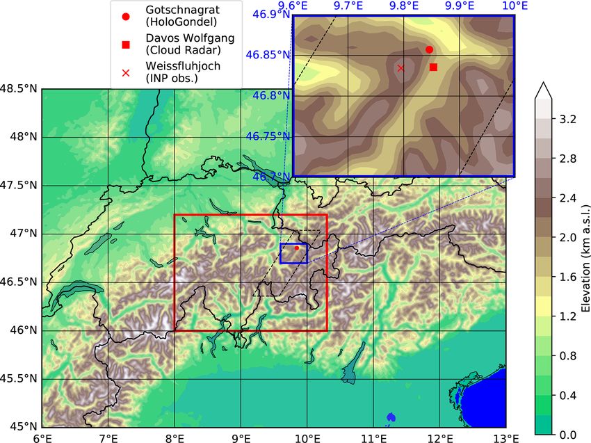
15116                                                                    Z. Dedekind et al.: Precipitation and secondary ice

(Blyth and Latham, 1997), e.g., when updrafts are less than        result of the collisional kinetic energy and was found to be
1 m s−1 for an integral ice crystal radius of 10 µm cm−3 (Ko-      most active at −15 ◦ C. Vardiman (1978) showed that colli-
rolev, 2007). To sustain MPCs, the supersaturation with re-        sional breakup occurs when large concentrations of rimed ice
spect to water must be maintained to compete with the deple-       crystals are present in convective clouds, which increases SIP
tion of water vapor by the depositional growth of ice particles    significantly.
(Korolev and Isaac, 2002; Bühl et al., 2016). In such environ-        Numerical formulations have been developed to describe
ments, supersaturation over liquid water is required so that       SIP by the collision of different ice species (e.g., Phillips
cloud droplets can grow in the vicinity of ice crystals. For ex-   et al., 2017a), e.g., when graupel collides with ice crys-
ample, mountainous regions can provide a continuous source         tals, when ice crystals collide with snow (e.g., Yano and
of liquid droplets through a constant air flow that is forced to   Phillips, 2011; Sullivan et al., 2018a) or when larger graupel
ascend due to the topography. In the Arctic regions, MPCs          collides with smaller graupel (Sullivan et al., 2017, 2018b;
can develop subcloud circulations leading to cold pool for-        Sotiropoulou et al., 2020). Therefore, the mass concentra-
mation and updrafts driving new convective cells (Morrison         tions of the collider species must be adequately simulated
et al., 2012; Lohmann et al., 2016a; Beck et al., 2018; Eirund     (e.g., Otkin et al., 2006), as any misrepresentation in the
et al., 2019a). Thus, the MPC lifetime is very sensitive to the    graupel category could potentially lead to significant differ-
updraft velocity (Korolev and Mazin, 2003; Lohmann et al.,         ences in the SIP rate. There are, however, only a small num-
2016a). Lohmann et al. (2016a) showed that high updraft ve-        ber of studies that have used these collisional breakup param-
locities, induced by steep orography, can stabilize a MPC. In      eterizations in mesoscale models (e.g., Sullivan et al., 2018a;
this case, the adiabatic cooling rate caused supersaturation       Hoarau et al., 2018; Sotiropoulou et al., 2020). Notably, Sul-
with respect to liquid water to exceed the diffusional growth      livan et al. (2018a) demonstrated that the lack of graupel
rate, allowing both cloud droplets and ice crystals to grow        formation in a cold frontal rainband in numerical simula-
(Korolev, 2007).                                                   tions compared to observations (Crosier et al., 2014) caused
   Primary production of ice crystals at temperatures warmer       collisional breakup to be 2 orders of magnitude less effec-
than the homogeneous nucleation threshold temperature              tive in SIP compared to rime splintering. Graupel was the
(−38 ◦ C) occurs through heterogeneous nucleation. The             only ice species that could cause collisional breakup when
number concentration of INPs can equal the ICNC in MPCs            it collided with either ice crystals or snowflakes. Another
at temperatures warmer than −38 ◦ C, when no secondary             possibility for SIP is droplet shattering upon freezing (e.g.,
ice production (SIP) process or external ice crystal sources       Kolomeychuk et al., 1975; Lauber et al., 2018). If the pres-
from the surface (e.g., hoar frost or blowing snow) or above       sure within a droplet reaches a critical point, the droplet may
(seeder–feeder process) are active. However, airborne ob-          fragment upon freezing. This process has been observed to
servations show that the ICNC can be orders of magnitude           happen for droplets larger than about 40 µm in diameter (e.g.,
larger than the INP concentration (Field et al., 2016, and ref-    Lawson et al., 2015; Korolev et al., 2020). The likelihood
erences therein). Field campaigns conducted at Jungfraujoch,       of fragmentation upon freezing and the number of produced
in the Bernese Alps in Switzerland, also showed that surface-      splinters during the fragmentation increases with droplet size
based measurements of ICNC exceed INPs by several orders           (Kolomeychuk et al., 1975; Lauber et al., 2018, 2021). In a
of magnitude (Henneberger et al., 2013; Beck et al., 2018).        modeling study, Sullivan et al. (2018b) showed that a warm
A modeling study conducted by Henneberg et al. (2017)              cloud base, between 20 and 25 ◦ C, at an updraft velocity of
over the Bernese Alps showed that simulated ICNCs dur-             4 m s −1 , is required for cloud droplets to grow large enough
ing winter are underestimated by an order of magnitude in          through coalescence or condensation to freeze and then shat-
MPCs as compared to the observations taken by Lloyd et al.         ter. As the cloud base temperature and updraft velocity de-
(2015). Temperatures were between −8 and −15 ◦ C and,              crease, droplet shattering becomes less efficient. Sullivan
therefore, too cold to trigger rime splintering, also known        et al. (2018a) could address the discrepancy between ICNC
as the Hallett–Mossop process (Hallett and Mossop, 1974).          and INP concentrations in their simulations by using the rime
Rime splintering occurs at warmer subzero temperatures, be-        splintering, collisional breakup and droplet shattering pro-
tween −3 and −8 ◦ C, and dominates ice multiplication in the       cesses simultaneously.
early stages of the cloud’s existence. However, a cold cloud          Several other mechanisms like hoar frost and blowing
base leads to slower diffusional droplet growth. In this case,     snow have been suggested as being surface flux processes
the cloud droplets remain smaller than the required 24 µm          that could lift ice particles from the surface of mountains and
in diameter that is needed for multiplication through rime         increase the ICNC of winter orographic MPCs (Rogers and
splintering (Hallett and Mossop, 1974). This cold cloud base       Vali, 1987; Farrington et al., 2016; Beck et al., 2018). Far-
could dampen the immense multiplicative nature of rime             rington et al. (2016) simulated ICNC at Jungfraujoch with a
splintering, revealing the dominance of other possible mech-       simplified parameterization for hoar frost. However, this pa-
anisms for multiplication early in a cloud’s existence, for        rameterization is independent of the surface concentrations
example, the collisional breakup of ice particles (Yano and        of hoar crystals, and including temporal variations in these
Phillips, 2011). The collisional breakup of ice particles is a     surface concentrations could improve the parameterization

Atmos. Chem. Phys., 21, 15115–15134, 2021                                          https://doi.org/10.5194/acp-21-15115-2021

Z. Dedekind et al.: Precipitation and secondary ice                                                                          15117

accuracy (Farrington et al., 2016). ICNC enhancement due
to hoar frost and blowing snow could also aid in enhancing
further SIP processes, but, currently, it is unknown which of
these processes dominates under different conditions. Under-
standing and representing the ICNC through the cloud, and
not only at the base of the cloud due to surface processes,
can also aid in obtaining a better representation of the sur-
face shortwave budget, particularly in the Antarctic (Young
et al., 2019). Independent of surface processes, hoar frost and
blowing snow, we are investigating the discrepancy between
ICNC and INP concentrations from the perspective of SIP
to examine two points. First, how active SIP processes are
in wintertime orographic MPCs, and whether they could ex-
plain the observed ICNC in a case study of the RACLETS
(Role of Aerosols and CLouds Enhanced by Topography and
Snow) field campaign. Second, what is the effect of SIP pro-
cesses on the cloud microphysics and, consequently, precip-       Figure 1. Overview of the model orography and the instrument lo-
itation formation, location and intensity?                        cation setup. The large domain is the simulated area that contains
                                                                  the analysis domain (red box). The enlarged blue domain is the lo-
                                                                  cation where measurements were taken during the RACLETS cam-
                                                                  paign. The parallelogram (dashed black lines) is the domain of the
2     Methods                                                     flow-oriented vertical cross section.

2.1    Case study of the RACLETS field campaign
                                                                  of HOLIMO 3G is 2D images of cloud particles, which can
The RACLETS campaign took place in February and March             be differentiated in ice and liquid particles for particles larger
2019 in the Davos region in Switzerland (also discussed           than 25 µm, depending on the shape of the ice particles (Hen-
in more detail in Lauber et al., 2021, and Ramelli et al.,        neberger et al., 2013). The separation between liquid droplets
2021a, b). Its goal was to improve our understanding of the       and ice crystals was done with a fine-tuned version of the
influence of both orography and aerosols on the development       neural network described in Touloupas et al. (2020), with
of clouds and on precipitation formation. Of particular in-       an overall uncertainty of the ICNC of ±10 %. Above that,
terest is that a cold front passed over the Swiss Alpine re-      the ice crystals were manually classified into irregular, pris-
gion on 7 March 2019 and was captured by measurements             tine, rimed and aggregated particles, which provides valu-
of precipitation and in situ measurements of cloud droplets,      able information on the precipitation formation process in
ice crystals and INPs. The precipitation rate and liquid wa-      orographic MPCs. Note that ice crystals can also be rimed
ter path (LWP) data were provided by the Leibniz Insti-           aggregates and, thus, fall into two categories. Because of the
tute for Tropospheric Research (TROPOS). The precipitation        total small number of recorded ice crystals
                                                                                                          √ and their different
rate was collected from rain gauge data when available, and       categories, the counting uncertainty ( N /V ; N – number of
otherwise from an upward pointing radar situated at Davos         crystals; V – measurement volume) was added to the overall
Wolfgang, 1630 m a.s.l. (above sea level) at a temporal reso-     uncertainty for the ICNC and for the different categories.
lution of 30 s. However, the radar attenuation from 08:15 to         HoloGondel was installed on a cable car on the Gotschn-
14:00 UTC was not corrected for. As a result, no estimation       abahn, which runs on the northwestern side of the ridge
of supercooled liquid within the MPC could be made. The           towards Gotschnagrat (2281 m a.s.l.), north of Davos Wolf-
LWP was estimated by the microwave radiometer that was            gang (see Fig. 1 for the exact location). HoloGondel took
situated at the same location as the radar. We also used the      in situ images of ice crystals and droplets within the cloud
precipitation data from MeteoSwiss in the form of a Com-          during three separate ascents of the Gotschnabahn running
biPrecip product, which is computed using a geostatistical        at the upper section between Gotschnaboden (1790 m) and
combination of radar estimates from plan position indica-         the Gotschnagrat mountain station (2280 m), specifically
tor radar data with rain gauge measurements (Sideris et al.,      at 11:54, 12:54 and 13:26 UTC on 7 March 2019. During
2014). We used CombiPrecip to capture the spatial extent of       these times, temperatures ranged between −2.8 and 0.7 ◦ C
precipitation over the Swiss Alps at an hourly resolution.        between Gotschnaboden and Gotschnagrat.
   Furthermore, ice crystal properties were collected using
the HoloGondel platform installed on the Gotschnabahn
(described in Lauber et al., 2021), which consists mainly
of the HOLographic Imager for Microscopic Objects 3G
(HOLIMO 3G in Beck et al., 2017). The outcome product

https://doi.org/10.5194/acp-21-15115-2021                                        Atmos. Chem. Phys., 21, 15115–15134, 2021
15118                                                                    Z. Dedekind et al.: Precipitation and secondary ice

2.2     Model setup                                                cation is appropriate in atmospheric models with a horizon-
                                                                   tal grid size and time resolution of 1x ≤ 1 km and 1t < 10 s
2.2.1    Spatial and temporal resolution                           respectively. Condensation and evaporation, represented by a
                                                                   saturation adjustment approach, are applied after the micro-
For the purposes of better understanding precipitation for-        physical conversion rates. The warm-phase autoconversion
mation, we used the non-hydrostatic limited-area atmo-             process from Seifert and Beheng (2001) was updated with
spheric model of the Consortium for Small-scale Modeling           the collision efficiencies from Pinsky et al. (2001) and also
(COSMO; Baldauf et al., 2011) version 5.4.1b. COSMO has            takes into account the decrease in terminal fall velocity asso-
recently been used to study wintertime orographic MPCs             ciated with an increase in air density. A better approximation
in the Swiss Alps (Lohmann et al., 2016a; Henneberg                of the collision rate between hydrometeors was also intro-
et al., 2017). The model domain roughly covers a region            duced by Seifert and Beheng (2006), which makes use of the
of 500 km × 400 km (45.5 to 49.5◦ N and 6 to 13◦ E) at a           root mean square values instead of the absolute mean values
horizontal grid spacing of 1.1 km×1.1 km (Fig. 1). For refer-      of the difference between the fall velocity of the colliding
ence, Davos Wolfgang is situated at 46.835◦ N and 9.85◦ E.         hydrometeors from the Wisner approximation (Wisner et al.,
A height-based hybrid smoothed level vertical coordinate           1972).
system (Schär et al., 2002) with 80 levels was used and               INPs available for immersion freezing are prognostic
stretched from the surface to 22 km. The applied orographic        throughout the simulations and are implemented following
smoothing at a horizontal resolution of 1.1 km×1.1 km re-          Possner et al. (2017) and Eirund et al. (2019b). The im-
duces the elevation of Gotschnagrat (located at 2300 m a.s.l.)     mersion freezing parameterization follows the DeMott et al.
to 1880 m a.s.l. For this study, we simulate the cold front pas-   (2015) temperature dependence and reproduces the deple-
sage between 07:00 and 14:45 UTC and analyze the results           tion and replenishment of INPs. The initial aerosol con-
between 09:30 and 14:45 UTC on 7 March 2019. Hourly ini-           centration for particles larger than 0.5 µm in diameter re-
tial and boundary conditions analysis data at a horizontal res-    quired for estimating the INP concentration was measured at
olution of 7 km × 7 km, supplied by MeteoSwiss, were used          Weissfluhjoch (2670 m a.s.l.) in clear air condition between
to force COSMO. The model time step was 4 s and the output         08:00 and 08:58 UTC on 5 March 2019. The days follow-
frequency every 15 min.                                            ing 5 until 7 March were cloudy, and an INP concentration
   Simulations were conducted with the SIP processes, where        was not measured. The average aerosol concentration larger
several SIP processes were active at the same time, and a          than 0.5 µm during this time was 3.32 cm−3 at an ambient air
control simulation (CNTL), where none of the SIP processes         temperature of 261 K (Seifert, 2019). Because of the tem-
was active. For each of these simulations, five ensemble sim-      perature mismatch between the observed temperature and
ulations are conducted by perturbing the initial temperature       the temperature range for which the INP parameterization
conditions at each grid point through the model domain with        is accurate (T < 258, DeMott et al., 2010), we used the re-
unbiased Gaussian noise at a zero mean and a standard devi-        trieved aerosol concentration from the upward-pointing lidar
ation of 0.01 K (Selz and Craig, 2015; Keil et al., 2019).         that was situated at Davos Wolfgang. The lidar retrieval gave
                                                                   a full vertical profile of the atmosphere. At temperatures be-
2.2.2    Cloud microphysics scheme                                 tween 258 and 243 K, the aerosol concentration larger than
                                                                   0.5 µm was between 1.8 and 2.5 cm−3 for which we then,
We use a detailed two-moment bulk cloud microphysics               accordingly, chose 2 cm−3 as input for the DeMott et al.
scheme within COSMO with six hydrometeor categories, in-           (2015) parameterization. At a temperature of 243 K, the es-
cluding hail, graupel, snow, ice, raindrops and cloud droplets     timated INP concentration was 23 L−1 . The freezing of all
(Seifert and Beheng, 2006). The two-moment bulk micro-             cloud droplets occurs at temperatures colder than 223 K. The
physics scheme has been used extensively to study the evo-         homogeneous freezing of cloud droplets, which is strongly
lution, lifetime, persistence and aerosol–cloud interactions       dependent on temperature, occurs at warmer subzero tem-
of MPCs (Seifert et al., 2006; Baldauf et al., 2011; Poss-         peratures. Another pathway of the liquid-to-ice conversion
ner et al., 2016; Lohmann et al., 2016a; Possner et al., 2017;     is the homogeneous nucleation of solution droplets that are
Henneberg, 2017; Glassmeier and Lohmann, 2018; Sullivan            typically associated with cirrus cloud formation. The formu-
et al., 2018a; Eirund et al., 2019a, b). We refer to ice parti-    lation of the homogeneous nucleation of solution droplets
cles as any combination of the hail, graupel, snow or ice cate-    follows Kärcher et al. (2006), which determines the number
gories. The size distributions of the hydrometeors, except for     density and size of nucleated ice crystals as a function of ver-
the raindrop category which is described by an exponential         tical wind speed, temperature and pre-existing cloud ice. A
distribution, are described by a generalized gamma distribu-       critical supersaturation must be reached in which nucleation
tion. Cloud droplet activation is based on an empirical ac-        events can occur if the updraft is stronger than a threshold
tivation spectrum which depends on the cloud base vertical         value determined by the radius and number density of the
velocity and the prescribed number concentration of cloud          pre-existing ice crystals (Eq. 19 of Kärcher et al., 2006). The
condensation nuclei (Seifert and Beheng, 2006). The appli-         freezing of raindrops occurs heterogeneously and indepen-

Atmos. Chem. Phys., 21, 15115–15134, 2021                                          https://doi.org/10.5194/acp-21-15115-2021
Z. Dedekind et al.: Precipitation and secondary ice                                                                               15119

dently of INPs. This is because the raindrop number concen-
tration is at least a factor of 103 smaller than the cloud droplet
number concentration and has an insignificant contribution to
the primary production of ice upon freezing (Figs. S4 and S5i
and j). It is included in our simulations because it is needed
for droplet shattering to occur. In the spectral partitioning of
freezing rain, only the frozen raindrops that are partitioned as
ice (Blahak, 2008) can cause multiplication through droplet
shattering, as discussed in the following section.

2.2.3   Secondary ice production parameterizations

Besides the primary ice formation pathways through ho-
mogeneous and heterogeneous nucleation, rime splintering
is the only process included in the standard version of              Figure 2. Secondary ice production processes at their defined tem-
COSMO that can enhance the ICNC otherwise. The rime-                 perature ranges. Panel (a) shows the probability of occurrence of
splintering process has been parameterized, implemented              droplet shattering (DS) and the triangular weighting function of
and tested in numerical weather models (Blyth and Latham,            rime splintering (RS). Panel (b) shows the fragment numbers gener-
1997; Ovtchinnikov and Kogan, 2000; Phillips et al., 2006;           ated by ice–graupel collisional breakup (BR) for the different cases
Milbrandt and Morrison, 2016; Phillips et al., 2017a). In            shown in Table 1. The red and yellow lines in (b) are the collisional
COSMO, rime splintering occurs exclusively after collisions          breakup parameterizations that were analyzed in the results.
between supercooled cloud droplets of diameter greater than
25 µm or raindrops with ice, snow, graupel or hail, all larger
than 100 µm (e.g., Seifert and Beheng, 2006), at temperatures        sizes of 83 and 310 µm. Droplet shattering in COSMO is
between −3 and −8 ◦ C (Hallett and Mossop, 1974). The pre-           parameterized as the product of a fixed fragment number,
dominant theory is that, within this temperature range, the          a temperature-dependent shattering probability given by a
supercooled droplets that rime on large ice particle freeze re-      normal distribution in temperature and the existing raindrop
sulting in a buildup of internal pressure whereby the pres-          freezing tendency used by Seifert and Beheng (2006). The
sure is relieved when the frozen shell cracks and produces           normal distribution is centered at 258 K, with a standard de-
3.5 × 10⁸ per kilogram of rime secondary ice particles (Hal-         viation of 5 K and a maximum probability of 10 % (as illus-
lett and Mossop, 1974). At temperatures colder than −8 ◦ C,          trated in Fig. 2a).
the ice shell of the frozen droplet is too strong to break              The collisional breakup of ice particles, in ice–ice colli-
(Griggs and Choularton, 1983), and at warmer temperatures            sions, was introduced and studied in laboratory experiments
than −3 ◦ C, the supercooled droplet spread over the ice par-        by Vardiman (1978) and Takahashi et al. (1995) and found to
ticle did not cause any SIP (Dong and Hallett, 1989). How-           be most effective at −15 ◦ C. Takahashi et al. (1995) enforced
ever, SIP has also been observed at temperatures outside the         the collision of large, 1.8 cm in diameter, heavily rimed ice
Hallett–Mossop droplet size and temperature requirements.            particles with one another and generated secondary ice parti-
   Droplet shattering produces maximum splinters at around           cles of up to 103 per collision. Yano and Phillips (2011) and
−15 ◦ C when large droplets freeze and shatter if the inter-         Yano et al. (2016) have demonstrated the generation of mas-
nal pressure buildup is high enough to eject fragments (e.g.,        sive enhancement of the ICNC by SIP due to ice–ice collision
Kolomeychuk et al., 1975; Leisner et al., 2014; Wildeman             in a dynamical system-type model. Recently, Phillips et al.
et al., 2017; Lauber et al., 2018; Keinert et al., 2020). So         (2017a) developed a more physically robust theoretical pa-
far, no temperature constraint is known for this process to          rameterization that was also applied in numerical simulations
be active below 0 ◦ C (Korolev et al., 2020; Lauber et al.,          that consider energy conservation. In our case, following Sul-
2021). The pressure buildup occurs mainly due to the unique          livan et al. (2018a), we take a more simplified approach. The
characteristic of liquid water having a higher density than          collisional breakup of ice particles in the laboratory work of
ice and, thus, expanding when it freezes. Larger droplets are        Takahashi et al. (1995) resulted in a temperature-dependent
more likely to shatter and likely produce more ice splinters         parameterization of the fragment number, as follows:
(Kolomeychuk et al., 1975; Lauber et al., 2018). However,                    FBR
                                                                                 (T − 252)1.2 exp −(T − 252)/γBR ,

as of yet, the number of splinters that are produced dur-            ℵBR =                                                            (1)
                                                                              α
ing droplet shattering could not be quantified. A more rig-
orous formulation for the fragment number remains a chal-
                                                                     ∂Nice
                                                                      ∂t     BR
                                                                                  = −ℵBR ∂N
                                                                                          ∂t
                                                                                             j
                                                                                                             ,                        (2)
                                                                                                  coll,j k
lenge due to the lack of measurement in laboratory studies.
Lauber et al. (2018) showed that the highest fragment rates          where α is the scale factor, FBR is the leading coefficient,
occur at around −15 ◦ C; however, this was only for droplet          T is the temperature in Kelvin, and γBR is the decay rate

https://doi.org/10.5194/acp-21-15115-2021                                            Atmos. Chem. Phys., 21, 15115–15134, 2021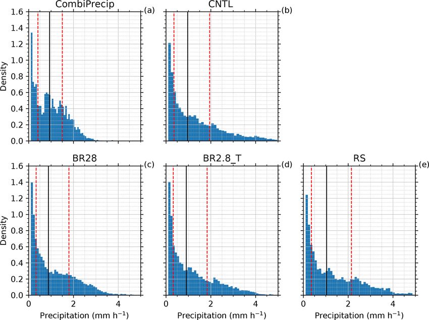
15120                                                                        Z. Dedekind et al.: Precipitation and secondary ice

Table 1. Sensitivity settings for the collisional breakup parame-    2016a). Korolev et al. (2020) identified midlatitude frontal
terization. α is the scale factor, FBR the fragments generated and   cloud systems within a temperature range of −15 and 0 ◦ C to
γBR the decay rate of the fragment number at warmer temperatures.    have 500 to 1000 L−1 small faceted ice crystals. Therefore,
Shown in bold is γBR = 5, as used by Sullivan et al. (2018a).        we increased the ICNC limit to 2000 L−1 in our model setup.
                                                                        Using droplet shattering as the only active SIP process
              α      FBR    γ BR = 5     γBR = 2.5                   in our case study yields very similar results to the CNTL
              4        70   BR70_T       BR70                        simulations, with the exception that the SIP rate between
              10       28   BR28_T       BR28                        4 and 5 km was 0.01 L−1 s−1 . The low SIP rate by droplet
              20       14   BR14_T       BR14                        shattering is because of the small rain mixing ratio at the
              100     2.8   BR2.8_T      BR2.8                       needed temperatures for this process. Therefore, it was not
                                                                     included in the rest of our analysis (Fig. S1 in the Supple-
                                                                     ment). Also, the initial analysis of the simulations with colli-
                                                                     sional breakup (for γBR = 2.5) showed that the SIP rate is be-
of fragment number at warmer temperatures. In our breakup            tween 1 × 10⁻³ and 7 L−1 s−1 below 5 km, yielding an ICNC
simulations, FBR and γBR are the experimental factors that           between 0.1 and 300 L−1 at the surface (Fig. S2a and g). Con-
are adapted for evaluating the collisional breakup parameter-        trasted against these simulations are the collisional breakup
ization. The fragment number ℵBR is multiplied by the colli-         simulations (for γBR = 5) that showed an increased SIP rate
sional tendency ∂Nj /∂t of the colliding hydrometeor pairs to        between 100 and 1000 L−1 s−1 , yielding ICNC of 2000 L−1
calculate the number of ice generated per time step ∂Nice /∂t        at the surface at Gotschnagrat (Fig. S3a and g). However, the
in Eq. (2). As shown in Fig. 2b, no collisional breakup oc-          ICNCs were strongly influenced by the upper bound of the
curs for temperatures below 252 K. Takahashi et al. (1995)           ICNC in COSMO, especially between 3 and 5 km. We chose
forced the collision between heavily rimed ice particles at a        the BR2.8_T settings because the observed ICNC was repro-
velocity of 4 m s−1 . However, when the collision speed from         duced best near the surface at Gotschnagrat in this simula-
the experiment is used to calculate the size of the involved         tion. Furthermore, the ICNC hard limit did not impact the
graupel particles, a 4 m s−1 fall speed corresponds to grau-         simulations, and therefore, collisional breakup and its im-
pel particles in the range of 2.5 mm in diameter according           pacts on the MPC can be understood better. Furthermore,
to Lohmann et al. (2016b). Considering the size–mass and             we used the BR28 simulation as a comparison to understand
fall–mass relations that are used in COSMO, Blahak (2008)            what the effect would be by reducing the SIP at warmer tem-
showed that, for graupel and hail falling at 4 m s−1 , the ef-       peratures than 263.5 K, while at the same time increasing
fective diameters were 4 mm and 1.4 mm, respectively. Also,          the SIP at colder temperatures than 263.5 K compared to the
in the simulations conducted here, graupel sizes would very          BR2.8_T settings (Fig. 2b). Higher ice particle number con-
rarely exceed 3 mm in diameter (not shown here). Therefore,          centrations at colder temperatures can increase the competi-
having smaller graupel particles than what was used in Taka-         tion for available cloud liquid water and glaciate the clouds
hashi et al. (1995), we expect ℵBR to be less, and thus, we          at a faster rate, slowing down precipitation formation. Due
introduce α to prevent extreme overestimations in ℵBR (Ta-           to their smaller size as a result of the aggressive collisional
ble 1). In contrast to Sullivan et al. (2018b, Table 1), graupel     breakup, these ice particles should have slower sedimentation
was the only species that could collide with and break up ice        velocities. We do expect that precipitation formation will be
or snow. Therefore, in our collisional breakup simulations,          slower in the BR28 simulations, and that there will be a lee-
hail was not permitted to collide with graupel and so reduce         ward shift in surface precipitation, assuming that the lower
the graupel diameter to smaller sizes, which emphasizes the          part of the MPC is supersaturated with respect to water.
need for α. Another consideration to take into account is that
COSMO treats snowflakes as unrimed particles, and as soon
as riming occurs on snowflakes, the snow mixing ratio is con-        3     Results
verted to the graupel mixing ratio, causing an especially large
graupel mixing ratio (Otkin et al., 2006). Since graupel is          3.1     Modeling ICNC and ice growth rates at
the only contributor to SIP through collisional breakup, in-                 Gotschnagrat
creased graupel mixing ratios could lead to excessive SIP.
Further sensitivity studies were conducted with γBR of 2.5           3.1.1    Modeling ICNC
instead of 5 as described in the parameterization used by Sul-
livan et al. (2018a). When γBR is 2.5, ℵBR will be reduced at        During each ∼ 2 min ascent, the HoloGondel platform on the
warmer temperatures (Fig. 2b).                                       cable car recorded ice crystal concentrations averaged over
   In the standard version of COSMO, the ICNC after each             three altitudes (1808–1961, 1961–2113 and 2113–2266 m).
model time step is limited to 500 L−1 for each level. How-           We first show the ICNC inferred from HoloGondel mea-
ever, measurements showed that the ICNC within MPCs                  surements on each of its three ascents (at 11:54, 12:54 and
produced higher ICNC of up to 1014 L−1 (Lohmann et al.,              13:26 UTC) and as the outcome of COSMO simulations at

Atmos. Chem. Phys., 21, 15115–15134, 2021                                            https://doi.org/10.5194/acp-21-15115-2021
Z. Dedekind et al.: Precipitation and secondary ice                                                                                   15121

Figure 3. HoloGondel measurements on 7 March 2019. (a) Total ICNC and measurement uncertainty (black error bars) of each gondola run
at each altitude. No measurements were taken at 11:54 UTC between 2113–2266 m and at 13:26 UTC between 1808–1961 m. (b) Irregular,
pristine, aggregated, rimed and rimed aggregate ice particles as the percentage of total ICNC averaged over the altitudes of each gondola run
are shown. The median temperature for each of the rides at the respective height, 1808–1961, 1961–2113 and 2113–2266 m, corresponds
to −1, −1.5 and −2.5 ◦ C, respectively.

Gotschnagrat (Fig. 1a). The total ICNCs from the observa-                10 and 12 L−1 , which compared better to the HoloGondel
tions were averaged over altitude for each ascent and were               observations, albeit with a high uncertainty below 3 km at
16 ± 5, 19 ± 4 and 9 ± 3 L−1 at 11:54, 12:54 and 13:26 UTC,              12:00 UTC. Differences in the ICNC profiles and specifi-
respectively. The simulated ICNC from the CNTL and rime-                 cally at the surface are to be expected between BR28 and
splintering simulations was less than 0.1 L−1 below 2.15 km              BR2.8_T because γBR controls the vertical ICNC profile.
for both 12:00 and 13:00 UTC (Figs. 4 and 5a) and was at                 However, in Fig. 4, there is a sharp decrease in the ice and
least 2 orders of magnitude smaller than the observations                snow mixing ratio, the depositional and riming rate and the
at Gotschnagrat (Fig. 3). Between 2.2 and 3.2 km, the SIP                cloud liquid between 2 and 3 km in altitude in the BR2.8_T
rate from rime splintering reached 5 × 10⁻³ L−1 s−1 (Figs. 4             simulation. It is likely that there was an inhomogeneity in
and 5g). Rime splintering originated exclusively from rain-              the MPC, acting as a sink to the mixing ratios and number
drops, with diameters between 150 and 250 µm at a con-                   concentrations and affecting the collisional tendencies and
centration of 0.1 L−1 that rimed onto ice particles (Fig. S4e            secondary ice production rates. The SIP rate of collisional
and o). A diameter of 25 µm required for rime splintering                breakup was 2 orders of magnitude larger than rime splin-
to be active was not met by the cloud droplets, which only               tering for 265 K ≤ T ≤ 270 K. The ICNC from collisional
reached diameters of 20 µm (Figs. 4 and 5f). The CNTL and                breakup was significantly larger than the CNTL simulation
rime-splintering simulations reached cloud droplet number                above 3 km. This process resulted in lower liquid water and
concentrations of 100 cm−3 and droplet diameters between                 rain mass mixing ratios, preventing primary ice production
10 and 22 µm, aiding in the primary ice production. The un-              because of the absence of liquid water (Figs. 4 and 5a–c
derestimated ICNC by the CNTL and rime-splintering sim-                  and g).
ulations emphasized the need to explore SIP with collisional
breakup.                                                                 3.1.2   Modeling ice growth rates
   The ICNC in the BR28 simulation, with reduced ice frac-
ture generation at warmer subzero temperatures, was be-                  The enhanced SIP through collisional breakup had a signifi-
tween 1 and 2 L−1 at 12:00 and 13:00 UTC (Figs. 4 and 5a),               cant impact on mostly glaciating the cloud above 2.5 km and
within an order of magnitude of the HoloGondel observa-                  can be seen in the nearly non-existent primary ice production
tions. The ICNC from the BR2.8_T was higher between                      rates due to the lack of cloud droplets (Fig. 4b and c). This
                                                                         also meant that the growth of ice was mostly through va-

https://doi.org/10.5194/acp-21-15115-2021                                               Atmos. Chem. Phys., 21, 15115–15134, 2021
15122                                                                           Z. Dedekind et al.: Precipitation and secondary ice

Figure 4. (a, e) Ice crystal number concentration (ICNC) and diameter, (b, f) cloud droplet number concentration (CDNC) and diameter,
(c, g) primary and secondary ice production and (d, h) riming and depositional (Dep.) growth of ice at Gotschnagrat at 12:00 UTC. The
solid lines are the model mean, with error bars showing the model spread for each simulation. The shaded regions are the minimum and
maximum values for the four closest model points. The mean ice diameter is denoted by IC. The green arrow is the average ICNCs from the
HoloGondel measurements (Fig. 3a).

Figure 5. (a, e) Ice crystal number concentration (ICNC) and diameter, (b, f) cloud droplet number concentration (CDNC) and size, (c, g) pri-
mary and secondary ice production and (d, h) riming and depositional (Dep.) growth of ice at Gotschnagrat at 13:00 UTC. The solid lines are
the model mean, with error bars showing the model spread for each simulation. The shaded regions are the minimum and maximum values
for the four closest model points. The mean ice diameter is denoted by IC. The green arrow is the average ICNCs from the HoloGondel
measurements (Fig. 3a).

Atmos. Chem. Phys., 21, 15115–15134, 2021                                                 https://doi.org/10.5194/acp-21-15115-2021

Z. Dedekind et al.: Precipitation and secondary ice                                                                            15123

por deposition that, in turn, suggests that the ice was mostly     Table 2. Vertically integrated growth rates (milligrams per square
unrimed and belongs in the irregular or pristine categories        meter per second; hereafter mg m−2 s−1 ) of ice over the lowest
above 2.5 km (Fig. 4d and h). Below 2.5 km, a very shal-           700 m at Gotschnagrat. In parentheses are the corresponding growth
low liquid layer that was subsaturated with respect to liq-        rate percentages.
uid water was present, causing ice particles to grow through
                                                                                         Gotschnagrat
the WBF process and/or riming at 12:00 and 13:00 UTC
                                                                    Simulation    Time     Riming         Deposition     Aggregation
(Figs. 4, 5a, b, d, f and S4d and e). The shallow mixed-                         (UTC)
phase cloud layer was of interest because, close to the sur-
                                                                    BR28         12:00     0.17 (0.2)    52.55 (80.3)    12.72 (19.5)
face the HoloGondel, observations showed that rimed par-            BR2.8_T                0.87 (2.6)    26.44 (80.5)     5.56 (16.9)
ticles were dominant, making up 47 %–72 % of the total
                                                                    BR28         13:00     4.35 (5.4)    47.11 (59.0)    28.38 (35.6)
ICNC, indicating that the cloud (at least close to the surface),
                                                                    BR2.8_T                8.56 (2.6)   154.87 (47.7)   161.67 (49.7)
from 11:54 to 13:26 UTC, was in a mixed-phase state while
passing over Gotschnagrat (Fig. 3b). Surprisingly, the rime-        BR28         13:30     0.43 (0.1)    90.36 (24.8)   273.96 (75.1)
                                                                    BR2.8_T                0.69 (0.1)   394.12 (52.9)   349.99 (47.0)
splintering simulation contributed little towards SIP, consid-
ering the large fraction of observed rimed particles (Figs. 3b,
4 and 5g). There are two possibilities for this discrepancy.
First, from the observations, the possibility exists that the      ice would have been either pristine or aggregated, whereas
recirculation of raindrops occurred, leading to additional         the ice crystal observations were predominantly rimed in the
breakup (Lauber et al., 2021). Ice particles that fall through     observations. Evidently, the cloud liquid water that acts as
the melting layer (∼ 1500 m; −1 ◦ C at 1808–1961 m; Fig. 3         rimers is underestimated in the collisional breakup simula-
caption) and melt to raindrops are lifted back into the MPC        tions. This analysis of the results could not be carried over to
by the turbulent mountainous flow. The increased in situ rain      the CNTL and rime-splintering simulations due to the un-
mixing ratio can provide additional rimer and, therefore, in-      derestimated ICNC. The ice that formed through primary
crease the number of rimed ice particles. Second, the low          ice production above 3 km sedimented through the overes-
SIP rate can be attributed to the lack of available liquid wa-     timated liquid layer (Fig. 6b) and grew by deposition and
ter in general, and when cloud droplets were present, they         riming (acting as a stronger sink to the ICNC), resulting in
were too small (less than 25 µm) to initiate rime splinter-        higher conversion rates from ice to graupel (Figs. 4 and 5b–d
ing (Hallett and Mossop, 1974). From the holographic im-           and h).
ages giving information on the ice particle size and habit,
the precipitation-forming processes can be inferred (Fig. 3a       3.2   Modeling precipitation
and b). Interestingly, observed irregularly shaped ice crys-
tals were also present that could have been artifacts from the     To analyze the impact of ICNC on precipitation, we com-
collisional breakup of ice or snow. However, it is also possi-     pared the cloud radar precipitation rate and the LWP
ble that the irregular ice crystals could either have originated   from the microwave radiometer with that of the simu-
from ice crystals that fell through different growth regimes,      lated precipitation rate and LWP. The observed precipita-
or they were from blowing snow and cannot be assigned to a         tion started at 08:30 UTC and continued until 14:00 UTC,
specific group (e.g., SIP). This would mean that only a frac-      reaching maximum precipitation rates over 15 min intervals
tion of the irregular ice crystals originated from the colli-      of 3.75 mm h−1 at 12:00 UTC as the cold front passed over
sional breakup.                                                    Davos Wolfgang. A total of 3 h of spin up was allowed be-
   Considering the lowest 700 m in the model, we calculated        tween 07:00 and 10:00 UTC; however, none of the simula-
the growth fraction of each of the growth mechanisms (rim-         tions was able to correctly simulate the onset of the pre-
ing, deposition and aggregation) of ice (e.g., riming (per-        cipitation. All the simulations underestimated the amount
cent) = riming/(riming + deposition + aggregation) from Ta-        of precipitation between 10:00 and 10:45 UTC (Fig. 6a).
ble 2). This was done to compare the ice crystal classifica-       After 10:45 UTC, the collisional breakup simulations over-
tion to the HoloGondel observations. This was not meant            estimated the precipitation as compared to observations.
to be a direct comparison because the ice in the model             Adding the rime-splintering parameterization also did not
could be rimed while also growing further by deposition,           improve the precipitation rate compared to the observations.
and vice versa, that could lead to double counting of pro-         This underlines the difficulty that models have in simulat-
cesses. However, following this approach, the BR2.8_T sim-         ing mountainous weather in general (Rotach and Zardi, 2007;
ulation showed that 2.6 %, 80.5 % and 16.9 % of the growth         Panosetti et al., 2018). The overestimation of the liquid wa-
was by riming, deposition and aggregation, respectively, at        ter path compared to the microwave radiometer was huge
12:00 UTC, compared to the BR28 simulation which showed            when the breakup of ice particles was excluded from the
growth fractions of 0.2 %, 80.3 % and 19.5 %. At 13:00 and         simulations. In general, including ice–graupel collisions sig-
13:30 UTC, the collisional breakup simulations experienced         nificantly reduced the liquid water path overestimation in
growth by riming of below 5.4 %, suggesting that most of the       the CNTL and rime-splintering simulations. The collisional

https://doi.org/10.5194/acp-21-15115-2021                                         Atmos. Chem. Phys., 21, 15115–15134, 2021
15124 Z. Dedekind et al.: Precipitation and secondary ice
Figure 6. Time series of (a) the precipitation rate from the rain gauge and cloud radar and (b) LWP from the microwave radiometer are
compared to all the sensitivity simulations at Davos Wolfgang. We interpolated the precipitation rate, LWP and LWF (liquid water fraction)
from the four closest model grid points to Davos Wolfgang. The shaded areas show the model spread for each simulation. Panel (c) shows the
LWF (percent) from 09:30 to 14:00 UTC on 7 March 2019. The observations, with their 30 s frequency, are integrated over 15 min intervals.
The model precipitation is accumulated over every 15 min.
breakup simulations, from 11:30 to 13:30 UTC, mostly un- Table 3. Interquartile range (IQR) between the 25th and 75th per-
derestimated the microwave radiometer liquid water path, centiles and median in millimeters per hour (hereafter mm h−1 )
which resulted in the MPC consisting of less than 10 % liquid for CombiPrecip and the sensitivity simulations and the Kullback–
water (Fig. 6b and c). Leibler divergences between CombiPrecip and the sensitivity simu-
As MPCs approach glaciation, precipitation formation lation precipitation distributions.
through the WBF process slows down when the updraft ve-
locity is not high enough to stabilize the MPC (Korolev IQR 25th 75th Median KL div.
perc. perc. (nats)
and Mazin, 2003). In the collisional breakup simulations, in
which the ICNCs were between 101 and 103 L−1 , the up- CombiPrecip 1.09 0.41 1.50 0.93
draft velocities were of the order of −0.2 to 0.6 m s−1 at al- CNTL 1.60 0.35 1.94 1.60 1163
titudes between 1.7 and 4.3 km. A liquid layer (cloud liquid BR28 1.46 0.33 1.79 1.46 930
water > 0.1 mg m−3 ) was present at the surface that extended BR2.8_T 1.51 0.32 1.83 1.51 1035
to approximately 1.6 km above the surface from 12:00 to RS 1.79 0.35 2.14 1.79 1132
13:00 UTC. Most of this layer, however, was subsaturated
with respect to liquid water, and the ice particle growth was,
via the WBF process, aided in precipitation formation. distances between asymmetric distributions was used. All
In Table 3, the integrated growth rates over the layer show the simulated precipitation distributions were more skewed
that a shift in growth rates in the layer were integrated over towards the tail, overestimating the density between 2 and
the lowest 1.6 km. 4 mm h−1 and underestimating the density between 1 and
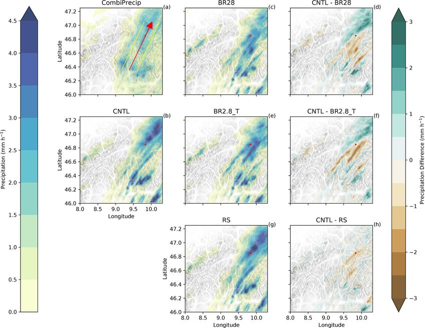
In Fig. 7, we consider the precipitation over the larger 2 mm h−1 over the domain. The collisional breakup simu-
domain (e.g., the red box in Fig. 1). The average wind di- lations diverge least from the observations, mainly due to
rection between 12:00 and 14:00 UTC, and between 2 and the lower and more accurate densities at higher precipita-
4 km above the surface, came from the southwest (indicated tion rates (Table 3 and Fig. 8). We calculated the interquar-
by the red arrow on Fig. 7a). To assess the skewed precipi- tile ranges with the 25th and 75th percentiles to compare the
tation distribution between the CNTL and sensitivity simu- precipitation distribution characteristics of the observations
lations, the Kullback–Leibler divergence that measures the with the simulations. CombiPrecip had a narrower precip-
itation distribution, indicated by the interquartile range be-
Atmos. Chem. Phys., 21, 15115–15134, 2021 https://doi.org/10.5194/acp-21-15115-2021Z. Dedekind et al.: Precipitation and secondary ice 15125 Figure 7. Precipitation rate (millimeters per hour; hereafter mm h−1 ) over the domain. (a) CombiPrecip, (b) CNTL, (c) BR28, (d) CNTL − BR28, (f) CNTL − BR2.8_T and (h) CNTL − RS. between 12:00 and 14:00 UTC. The yellow lines are the outer limits of the cross sections around the red arrow showing the wind direction. The red marker shows the location of Gotschnagrat, and the gray shading is the topography between 0 (white) and 3700 m (dark gray). tween the 25th and 75th percentiles of 1.09 mm h−1 , than all dated over flat terrain (e.g., Mellor and Yamada, 1982; Ro- the simulations, meaning that the observed precipitation was tach and Zardi, 2007), which is not the case for our study. less variable. This can be seen in the domain as all the simu- As a result, the 1D turbulence scheme can underestimate lations had regions of localized high precipitation rates. This the subgrid-scale variability in the vertical velocity. Earlier resulted in a higher variability, with an interquartile range be- and higher precipitation rates can occur if the mountains are tween 1.46 and 1.79 mm h−1 , of which 75 % of the precipita- high enough to force the flow into an elevated mixed layer, tion was between 1.7 and 2.14 mm h−1 (Fig. 8). The localized leading to a faster transition of deep convection (Panosetti regions of stronger convection and invigorated precipitation et al., 2018). From a microphysics point of view, the ice par- when the SIP processes were excluded, causing the higher ticles in the CNTL simulation are not multiplied through SIP variability, can most likely initially be attributed to the dy- and, therefore, can rapidly grow large, sediment out of the namics. The microphysics scheme then further enhanced the cloud at faster rates and overestimate the surface precipita- precipitation overestimation in the localized regions. Craig tion (Figs. 4e and 5e). and Dörnbrack (2008) demonstrated that a model resolu- The localized regions of invigorated precipitation rates tion of ∼ 1 km is approximately equal to the characteristic were suppressed by including the SIP processes (e.g., three turbulence scales of convective structures. Therefore, using cases are shown in Figs. S6 and S7). Because collisional a 1D turbulence scheme, which we used and is generally breakup is a mechanical process, it does not contribute di- used in cloud-resolving models, is not optimal and in the rectly to the latent heat budget and, therefore, should not “gray zone”. Also, horizontally homogeneous conditions are invigorate the updraft velocities. However, larger number assumed in most turbulence schemes and have been vali- concentrations of ice particles can cause increased deposi- https://doi.org/10.5194/acp-21-15115-2021 Atmos. Chem. Phys., 21, 15115–15134, 2021
15126                                                                      Z. Dedekind et al.: Precipitation and secondary ice

Figure 8. Precipitation rate (mm h−1 ) histogram for (a) CombiPrecip, (b) CNTL, (c) BR28, (d) BR2.8_T and (e) RS from the domains in
Fig. 7. The median (black solid line) and the 25th and 75th percentiles (red dashed line) are shown.

tional growth and, thereby, change the buoyancy structure           not too wide so that the results become diluted. The MPC
of the cloud (Fig. S7). Stronger updrafts could then loft the       was defined by cloud droplet and ice mixing ratios greater
smaller ice particles to higher altitudes, reducing their sed-      than 10 and 0.1 mg m−3 , respectively. In the CNTL and rime-
imentation velocities towards the surface. Evidence for the         splintering simulations, the mixed-phase part of the cloud ex-
effect of the strong SIP rate on ice particle size can be seen      tended to approximately 5 to 6 km and had a cloud top at
in Figs. S4 and S5k–m. The BR28 simulation, which was               234 to 235 K. The rime-splintering rate below 4 km was con-
able to produce the largest SIP rates, resembled the mag-           fined to 0.1 L−1 s−1 , with the highest primary ice production
nitude of the precipitation CombiPrecip the best by reduc-          rate of 0.01 to 0.1 L−1 s−1 between 4 and 7 km. The structure
ing more of the localized high precipitation regions of the         of the MPC did not change significantly due to the enhanced
CNTL simulation (e.g., Figs. 11 and S6). To the north of            SIP from rime splintering. The additional ice formation near
Gotschnagrat, the cloud was mostly glaciated, slowing pre-          the surface in the vicinity of the abundant cloud liquid wa-
cipitation down (Fig. 7c, f and i). Over the domain, the            ter caused a significant increase in the averaged depositional
spread of the precipitation between the 25th and 75th per-          growth rates over the cross section from 1.72 to 2.20 g m−2
centiles was 1.46 mm h−1 , with 75 % of the precipitation be-       (an increase by 28 %), while the riming rates also showed a
low 1.79 mm h−1 (Fig. 7c and d and Table 3). Another inter-         small increase (Figs. 9d and 10e and f). Higher mass mixing
esting feature is that the rime-splintering simulation caused       ratios in snow and graupel, also reflected in the higher ice
a southward shift in the precipitation when compared to the         water fraction, were produced as a result of the faster con-
CNTL simulation (Figs. 7b and h and 10g).                           version from ice (Fig. 10a and c). This led to earlier and in-
                                                                    creased surface precipitation upstream of the flow direction
3.3   SIP impact on precipitation over the flow-oriented            over that of the CNTL simulation (Fig. 10g).
      cross section                                                    Collisional breakup had a distinct effect on the MPC, re-
                                                                    ducing its vertical extent to around 4 km (Fig. 9b and d). In
The flow-oriented vertical cross section, as depicted in Fig. 7,    both of the collisional breakup simulations, the SIP reached
helps to explain the behavior of the MPC with respect to            100 L−1 s−1 below 5 km, impacting the primary ice produc-
enhanced SIP (Fig. 9). The width of the cross section is            tion rate strongly due to the significant reduction in the LWP
∼ 25 km, covering a majority of the precipitation along the         (Figs. 9b and 10d). As a result, there was a clear shift towards
cross section, as seen in the observations. It was chosen along     the depositional growth of ice particles from 46.4◦ N north-
the average wind direction during the analysis period, mak-         wards. Korolev and Mazin (2003) showed that, for high val-
ing it wide enough for robust results and, at the same time,        ues of Ni r i and updraft velocities between 0.1 and 1 m s−1 ,

Atmos. Chem. Phys., 21, 15115–15134, 2021                                            https://doi.org/10.5194/acp-21-15115-2021
Z. Dedekind et al.: Precipitation and secondary ice 15127 Figure 9. Primary ice production and secondary ice production (per liter per second; hereafter L−1 s−1 ) averaged between 12:00 and 14:00 UTC for (a) CNTL, (b) BR28, (c) BR2.8_T and (d) RS. The hatched area is defined as the MPC where the cloud droplet mass concentration and ice mass concentration is greater than 10 and 0.1 mg m−3 , respectively. The pink line is the homogeneous freezing line at 235 K, and the shaded gray area is the cloud area fraction. Figure 10. (a) Graupel water path, (b) IWP (ice water path), (c) IWF (ice water fraction) (IWP/(IWP + LWP)) × 100, (d) LWP, (e) riming rate and (f) deposition rate over the cross section. These quantities calculated in panels (a)–(f) were only over cloudy regions, where the cloud area fraction is larger than 0. In parentheses are the average over the latitude. Panel (g) shows the precipitation mean (solid line), ensemble spread (shaded area) and CombiPrecip (dashed line), and panel (h) shows the averaged topography over the cross section. The red vertical dashed line indicates the latitude of Gotschnagrat. https://doi.org/10.5194/acp-21-15115-2021 Atmos. Chem. Phys., 21, 15115–15134, 2021
15128                                                                           Z. Dedekind et al.: Precipitation and secondary ice

Figure 11. Schematic summary of the impact of collisional breakup of ice particles on the cloud structure and surface precipitation.

the ice particles will absorb water vapor rapidly, reducing it          and BR2.8_T, respectively, compared to the rime-splintering
to saturation over ice and, therefore, controlling the supersat-        simulations of less than 0.1 L−1 . The BR28 simulation most
uration. Stronger combined growth rates of up to 33 % com-              closely reproduced observations, albeit leading to ICNC an
pared to the CNTL increased the latent heat release, updraft            order of magnitude smaller than observed at Gotschnagrat.
velocities and, ultimately, precipitation over the cross section        However, blowing snow cannot be excluded as a contribu-
between 46.5 and 46.8◦ N. The BR2.8_T simulation, espe-                 tor to the measured ICNC (e.g., Farrington et al., 2016; Beck
cially, overestimated the precipitation because of the higher           et al., 2018; Walter et al., 2020) even though we were not
SIP rates at warmer temperatures in the vicinity of cloud               able to quantify this process in our analysis. The resuspen-
liquid water (Figs. 9c and 10g). North of 46.7◦ N, the IWF              sion of snow particles from the surface into the atmosphere
was well above 95 %, glaciating large parts of the MPC. Be-             where they could potentially interact with cloud particles is
cause of the loss of cloud liquid, precipitation formation was          dependent on the wind speed. The total mass change of the
slowed down, reducing the surface precipitation windward of             snow pack is a function of the horizontal distribution of blow-
Gotschnagrat (Fig. 10c to g). This resulted in a mean precip-           ing snow, the sublimation rate of blowing snow, the sublima-
itation rate over the cross section that was 2 mm h−1 com-              tion/evaporation rates or condensation/deposition rate at the
pared to CombiPrecip at 1.69 mm h−1 . The BR2.8_T precip-               surface, the precipitation rate and the runoff of liquid water
itation intensity lags behind that of the BR28 simulation over          that all impact the mass change rate of a snowpack (Arm-
the flow-oriented vertical cross section (Fig. 10g). The faster         strong and Brun, 2008). Mahesh et al. (2003) have found
precipitation formation is coupled to the higher ICNC within            that a threshold value for the wind speed above ∼ 7.6 m s−1
a MPC that can enhance riming, as long as liquid droplets are           is necessary to resuspend snow particles. More recently in
present, or else by the WBF process. The precipitation mag-             the Swiss Alps, Walter et al. (2020) interpolated a threshold
nitude in the BR28 simulations matched the observed precip-             value of ∼ 7.5 m s−1 from radar observations, which was in
itation better but was shifted towards the south. In summary,           agreement with other studies (e.g., Li and Pomeroy, 1997).
we have provided evidence that COSMO may benefit from                   Wind speeds of larger than 7.5 to 15 m s−1 could then trans-
the inclusion of collisional breakup processes in simulating            port these snow particles over distances of 60 to 240 m. In our
ICNC and precipitation.                                                 case, the wind speeds recorded by the snowdrift station used
                                                                        by Walter et al. (e.g., 2020) were mostly below the 7.5 m s−1
                                                                        for the largest part of our analysis period (Fig. S8). However,
4   Discussion                                                          between 12:45 and 13:30 UTC when wind speeds exceeded
                                                                        7.5 m s−1 , a case can be made for blowing snow affecting the
Our study suggests that including SIP through collisional               ice particle number concentration in the MPC and, thereby,
breakup can enhance the in situ ICNC and, consequently, sur-            triggering secondary ice processes. As a consequence, the
face precipitation. The collisional breakup simulations led to          current discrepancy in ICNC between the collisional breakup
ICNCs at Gotschnagrat of 1 to 2 orders magnitude larger than            simulations and the observations could be overestimated.
in the rime-splintering simulations. More precisely, the num-              Surprisingly, our SIP rate through collisional breakup was
bers were between 1 and 2 L−1 and 10 and 12 L−1 for BR28                between 104 and 106 times larger than what Sullivan et al.

Atmos. Chem. Phys., 21, 15115–15134, 2021                                                 https://doi.org/10.5194/acp-21-15115-2021
You can also read