Mode and tempo of cultural evolution in video games - Ivan Dmitriy Ortiz Sánchez - e ...
←
→
Page content transcription
If your browser does not render page correctly, please read the page content below
BACHELOR´S THESIS / BIOMEDICAL ENGINEERING 2021

                                                  Mode and tempo of cultural evolution in
                                                  video games

                                                  Ivan Dmitriy Ortiz Sánchez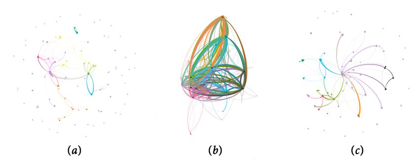
Mode and tempo of cultural evolution in
              video games

          Ivan Dmitriy Ortiz Sánchez

         Bachelor’s Thesis UPF 2020/2021

                     Thesis Supervisors:

Dr. Sergi Valverde Castillo,   (Evolution of Technology Lab, CSIC-UPF)

Dr. Salvador Duran Nebreda,     (Evolution of Technology Lab, CSIC-UPF)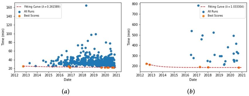
Dedicatory

             To my family, for their unconditional presence and trust.

  To my friends and beloved, for being so far yet so close in such a different year.

          Finally, to Juan Ortiz and to Isabel Peñarroya. In Memoriam.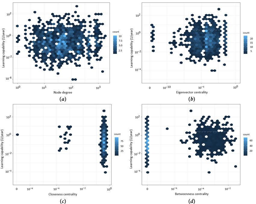
Acknowledgments
I would like to wholeheartedly thank my supervisors, Sergi and Salva, and acknowledge
their help, advice and patience during this research. It has been a fascinating and worth-
while experience and, without their time and enthusiasm, this study would have not been
the same. I am also thankful for all the knowledge about cultural evolution and network
theory and the computational methods they have taught me during the research, which
have given me a better comprehension of such a beautiful and engaging field of research.
Summary/Abstract
The mechanisms of biological evolution also apply to artificial phenomena such as culture
and technology, and the evolution of video games through history has been shaped by
the evolution of technology itself. In particular, the so-called speedruns, which consist
in completing video games in the least time possible, have become remarkably popular
recently. Since the evolution of performance in video games has never been quantita-
tively assessed, in the present study, we wonder whether there are universal patterns in
the way speedrunning has evolved through video game history. Specifically, we aim to
identify relations between performance improvement and the size and structure of the
player community. Thus, a reliable dataset with the results of official speedruns has been
manipulated and analyzed. First, we describe the dynamics of performance improvement
and growth of the community since its origin. Second, we explore the effects of commu-
nity structure with a game-player bipartite network framework and an infectious model
of strategy and information propagation. Finally, we relate the model to the actual data
and establish linkages between the properties of the network and the learning dynamics.
Our results show how the growth of the community and the evolution of performance
follow exponential descriptions and how the rank-ordered distribution of players accord-
ing to their number of playthroughs follows a power law-like behaviour. A first minimal
network model to describe the properties of the community is also provided. This study
lays the foundation for a quantitative application of biological and evolutionary models
to the video game field.

Keywords
computational modelling, complex networks, infection models, cultural evolution, learn-
ing, video games, speedrunning
Preface
The evolution of video games has been shaped by the evolution of technology itself, and,
in the current context, video games are highly influential. The relevance of the role they
play in our society, not only for the youth but for people of all ages, especially with the
rise of streaming platforms and the so-called speedrunning community, is undeniable.

Cultural patterns are evolutionary, and those mechanisms which define biological evo-
lution have been proven to work with cultural phenomena as well, and allow to either
understand the past or forecast the future. Given the mathematical tools and the biologi-
cal concepts learnt through the Biomedical Engineering degree, an application of cultural
evolution methods to the video game field in order to assess how it has changed through
time would represent a first insight into the topic from an evolutionary perspective, and
a relevant scientific contribution.

Given this context, we are motivated to explore video game performance and the structure
of the community of players and to try to identify universal patterns in the way they have
evolved which could be explained by means of simple mathematical descriptions, and to
provide a basis for further analyses in such an unexplored and relatively novel area.
Index
1 Introduction 1
2 Stage I. Evolution of speedrunning and video game performance 6
2.1 Methods . . . . . . . . . . . . . . . . . . . . . . . . . . . . . . . . . . . . . 6
2.1.1 The data set . . . . . . . . . . . . . . . . . . . . . . . . . . . . . . . 6
2.2 Results . . . . . . . . . . . . . . . . . . . . . . . . . . . . . . . . . . . . . . 6
2.2.1 A DGBD model for cultural evolution in video games . . . . . . . . 6
2.2.2 An exponential decay model for performance improvement . . . . . 10
3 Stage II. A minimal model for the structural growth of the community 12
3.1 Methods . . . . . . . . . . . . . . . . . . . . . . . . . . . . . . . . . . . . . 12
3.1.1 The model . . . . . . . . . . . . . . . . . . . . . . . . . . . . . . . . 12
3.1.2 Structural analysis of the community . . . . . . . . . . . . . . . . . 15
3.2 Results . . . . . . . . . . . . . . . . . . . . . . . . . . . . . . . . . . . . . . 18
3.2.1 Properties of the community as a network . . . . . . . . . . . . . . 18
3.2.2 Graph visualization . . . . . . . . . . . . . . . . . . . . . . . . . . . 23
4 Stage III. Community structure and learning capability of players 25
4.1 Methods . . . . . . . . . . . . . . . . . . . . . . . . . . . . . . . . . . . . . 25
4.1.1 Learning capability as a node-specific property . . . . . . . . . . . . 25
4.2 Results . . . . . . . . . . . . . . . . . . . . . . . . . . . . . . . . . . . . . . 25
4.2.1 Influence of learning capability on the community . . . . . . . . . . 25
4.2.2 A structural transition in time . . . . . . . . . . . . . . . . . . . . . 27
5 Discussion 28
Bibliography 31
Supplementary information 33
S.I Generation of multiple components in simulations . . . . . . . . . . . . . . 33
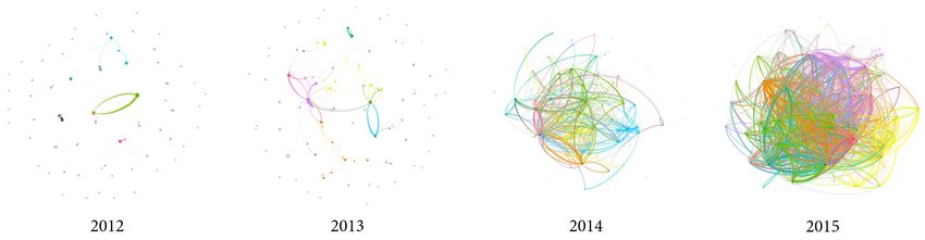
S.II Learning capability . . . . . . . . . . . . . . . . . . . . . . . . . . . . . . . 34List of Figures 1 Growth in the number of speedruns and player productivity . . . . . . . . 7 2 Rank-ordered distribution of players and DGBD fit . . . . . . . . . . . . . 8 3 Rank-ordered distribution of games and DGBD fit . . . . . . . . . . . . . . 9 4 Example of evolution of performance in a video game . . . . . . . . . . . . 10 5 Probability density of learning rates . . . . . . . . . . . . . . . . . . . . . . 11 6 Rank-ordered distribution of players and games; empirical and simulated . 15 7 Node degree occurrence distribution . . . . . . . . . . . . . . . . . . . . . . 19 8 Average node degree in projections . . . . . . . . . . . . . . . . . . . . . . 20 9 Centrality occurrence distribution in bipartite graphs . . . . . . . . . . . . 21 10 Centrality occurrence distribution in projections . . . . . . . . . . . . . . . 21 11 Global efficiency of communities . . . . . . . . . . . . . . . . . . . . . . . . 22 12 Number of edges and modularity in projections . . . . . . . . . . . . . . . 22 13 Connectance of communities . . . . . . . . . . . . . . . . . . . . . . . . . . 23 14 Graph visualization: real and simulated . . . . . . . . . . . . . . . . . . . . 23 15 Learning capability and node-specific properties of the community . . . . . 26 16 Graph visualization: community evolution between 2012 and 2015 . . . . . 27 S1 Graph visualization: comparison in terms of ρ . . . . . . . . . . . . . . . . 33 S2 Mean learning rate and node-specific properties of the community . . . . . 34 S3 Influence of players with zero learning capability . . . . . . . . . . . . . . . 35
List of Tables
No tables have been included in this document.
1    Introduction
The evolution of living beings is characterized by certain mechanisms which act in favour
of the survival of those organisms who are better adapted to the environment, namely
reproduction (and inheritance of genetic traits), mutation and selection, principally. Re-
production allows the persistence of living beings through multiple generations, mutation
is a source of randomness and, thus, allows to introduce change and innovation. Crossover
between individuals with different characteristics also allows to obtain variability. Finally,
selection is a natural mechanism by means of which the environment tests living beings’
condition and adaptability and allows to survive only those with the proper character-
istics. Evolution does not only allow life to persist in time but also to generate a large
variability of species (and even between individuals of the same species) and organisms
with high complexity.

Given the potential of these natural mechanisms, the human being has wondered whether
they could be applied to artificial processes, systems and dynamics. Examples of these
are the so-called evolutionary algorithms or the evolution of human culture. Evolutionary
algorithms use the concepts of reproduction, mutation, crossover, selection, migration,
etc. to find optimal solutions to a given problem. On the other hand, it is shown that
human culture is itself an evolutionary process exhibiting those mechanisms which define
Darwinian evolution [1].

Culture can be defined as group-typical behaviour patterns shared by members of a com-
munity that relies on socially learned and transmitted information [2, 3]. In cultural
evolution, apart from culture itself, the concept of cumulative culture is also important,
which refers to the fact that cultural traits are based on the legacy from previous gener-
ations and the knowledge about that legacy [4]. Hence, cumulative culture means that
culture can be spread through generations and grow, but it also depends on the population
itself, since cultural traits must be learned properly in order to avoid losses through time.
Cumulative culture also implies that the accumulated knowledge overcomes what a single
individual would manage to invent on his or her own [5]. The accumulation of culture is
also a punctuated process: remarkable innovations might appear after uninterrupted long
technologically stable periods [3]. When a large number of innovations appear together or
in rapid succession at a certain time or place, it is said that a technological transition has
occurred [6, 7]. Nevertheless, not many innovations manage to represent turning points
in human culture; in human history, only milestones such as the apparition of language
or the invention of computers manage to generate such discontinuities.

Network studies have developed multi-layered models in which nodes can either be indi-
viduals, communities or even a certain type of cultural trait [3, 6, 8]. It has been shown
that those cultural structures in which nodes are densely connected tend to manifest
higher levels of transmission or learning rates than those which rather have high modu-
larity. However, modularity allows to increase cultural variability and innovation [8, 9].
As a summary, it can be stated that the higher the community size and its variability,
and the more communication between the individuals, the easier the overall learning or
performance and maintenance of cultural traits [10, 11, 12].

Cultural transmission, however, also has barriers which might constrain the process, or

                                                                                            1
even lead to cultural loss, which can either be structural or behavioural [13]. Structural
barriers are directly related to the network itself, by means of affecting the contact be-
tween individuals. On the other hand, behavioural constraints depend on the willingness
of individuals to share and spread their knowledge. Through generations, there is also a
certain degree of inaccuracy in cultural transmission, since information can be misunder-
stood or not properly shared.
In cultural evolution, many studies use the so-called neutral models, in the sense that the
dynamics have been assumed to rely on a certain stochasticity which can be controlled
or defined by certain constant parameters, providing simple approaches to explain quite
complex systems [14]. However, there is certain controversy on whether neutral models
are conclusive or not, since they are criticized for considering deterministic processes such
as adaptation or selection as merely stochastic [14]. Nevertheless, it is also defended that
chance and stochasticity are not sufficiently considered in cultural evolution, and that
certain collective decisions can statistically behave as if the product of random copying,
which would justify the suitability of stochastic models [15].
Minimal models for technological diffusion have been proposed in which the technological
level is a variable that improves in a fashion proportional to the size of the community
(which increases in a logistic manner) and decreases due to a certain transmission error
[6]. Such models have two stable states: low population with low cultural level and high
population with high cultural level. This mechanism applies for urban phenomena, for
instance: certain urban features increase faster according to the size of the population
[16, 17]. These systems show a positive feedback mechanism in which the wise become
wiser and those with the least cultural level might even become extinct.
The use of models of this kind has allowed to establish patterns in the evolution of cer-
tain cultural traits or to forecast technological progress as well as to provide frameworks
for the analysis of such traits [3, 18]. These models have provided mathematical tools
in the shape of simple equations based on relations such as exponential or power laws,
which allow a better comprehension of the past and to make predictions about the fu-
ture. Cultural evolution studies can thus be applied either to archaeology or to current
technological dynamics, and one cultural area that could be of particular interest in the
current context is the field of video games.
Video games play a very relevant role nowadays in society. Even though they might
be thought as a mere source of entertainment, there are at least three different aspects
in which their actual importance can be reflected, namely socioeconomic, cognitive and
technical.
First, the economic and social impact of video games must be born in mind. As a matter
of fact, the global video game market size was valued at 151.06 billion US dollars in 2019
and it is expected to grow at a compound annual growth rate (CAGR) of 12.9% from
2020 to 2027 [19]. The social importance of video games can be observed in the growth of
the so-called speedrunning community, considered in this study. The recent growth of the
video game community regardless of speedrunning can also be explained as a consequence
of the rise of platforms such as Twitch, YouTube and Discord, which allow to stream and
2spread information about video games.1,2,3 Furthermore, certain video games have also
contributed to different economic areas such as cinema, literature or other merchandise
thanks to their fame.
Second, video games have been reported to have a beneficial effect on human cognition. A
causative relationship has been observed between video game play and augmented spatial
resolution [20]. It has also been possible to establish linkages between neural and cognitive
aspects regarding attention, cognitive control, cognitive workload, and reward processing
[21]. These results have led to the use of video games as therapeutic tools, since the effects
on cognition are reflected in brain structure and function. However, no strong scientific
evidence about the underlying mechanisms in the brain has been reported when it comes
to supporting the clinical application of video games [22].
Finally, a technical factor should be considered: the process of developing a video game
involves the integration of a wide range of professionals and fields, such as computer pro-
gramming, economic and business management, arts (auditory, visual, narrative, etc.) or
marketing.
Hence, the fact that no previous studies on cultural evolution have been conducted in
such a relevant field provides the opportunity to perform a first insight into the topic,
and to try to establish a first theoretical basis for further research and analysis about the
evolution of performance in video games.
Given this scenario, we hypothesize that there might be universal patterns in the way
video game performance and the community of players have evolved through video game
history. Specifically, we aim to (1) assess the cultural growth of the video game com-
munity, (2) analyze its structural properties, and (3) identify possible relations between
the rate of improvement and the size and structure of the community of players. Given
these three main goals, and the fact that each of them requires the results from the steps
followed to achieve the previous one, this study is organized in three different stages which
have been treated independently, each one with different methods and strategy, which aim
to fulfil each objective.
In order to assess performance in video games, this study is focused on analysing the
so-called speedruns, which consist in finishing games in an optimal manner. We consider,
then, that the ideal parameter to measure optimality is the time required to complete a
game. It must be noticed that speedrunning does not consist in playing as fast as possible
per se without a deep understanding of each game but in uncovering and deciphering
as much information as possible on how the game is designed and programmed so that
players can take advantage of it and find shortcuts, strategies or a priori unexpected tech-
niques to reduce the time taken to complete it. This procedure is known as routing.
Since there is a large number of video games as well as a wide range of genres, it should
be expected that each of them could be treated in a different manner. However, as
previously stated, this study takes the following assumption: optimality in video game
1
www.twitch.tv
2
www.youtube.com
3
www.discord.com
3performance can be universally assessed measuring the time taken to complete a game.
This justifies why speedrunning data is the best source of information about performance.
Furthermore, each video game might have different strategies or ways to be completed. In
general, most video games are considered to be completed once the ending credits appear
(or right when the last movement before the game finishes is performed). Thus, part of
the content of a game can be skipped during a run, that is, a complete playthrough. This
is why each game has different categories. The most typical categories are the so-called
“Any%”, “100%” and “Low”. The first one aims to complete a game as fast as possible.
The second one aims to complete all the content it has to offer. Finally, the Low mode
aims to complete the game avoiding as much collectable items as possible. The difference
between Any% and Low is that in the first one the number of items gathered does not
matter, but they might coincide in certain cases. Hence, Any% is the category in which
the lowest scores are achieved. Note that scores between different categories are indepen-
dent. A single video game might include other categories than the aforementioned, and
they might be due to its individual design, genre or style, for instance. For each category,
however, certain rules are set, and they must be respected by all players. Other remark-
able categories are the “Glitchless” mode, which does not allow techniques that break a
video game’s original rules, or those other categories which rely on minimizing the num-
ber of “presses” of a certain button during the run, that is, executing a specific command
(e.g. jumping, moving to a specific direction, running, shooting, etc.). Finally, there also
exists a special sort of speedruns, which are the so-called Tool-Assisted Speedruns (TAS ).
Many video games, in order to be completed in the least amount of time, involve certain
mechanisms which require too much accuracy for a person. Consequently, even if an in-
dividual managed to perform them, it could be considered the result of luck or after an
unimaginable number of attempts. Tool-Assisted Speedrunning aims to solve this limita-
tion: players do not perform the run but make a computer program execute the run itself.
Thus, players analyze and specify each single movement and command frame by frame in
order to reach optimal performances. Even though TASs rely on the users’ ability, they
do not involve an actual person playing the video game. This is why they can be used to
set theoretical perfect scores to video games, but not as actual human runs. Furthermore,
non-tool-assisted speedruns can be performed in real time (Real Time Attack ) without
stops, or in a segmented manner, dealing with the stages of a video game separately and
then summing the best scores.
In order to perform this study, a reliable dataset registering scores for a total of 4,962 dif-
ferent categories from 693 different video games is manipulated and analyzed. This dataset
is provided by a world-wide known speedrunning website (speedrun.com), in which video
game players share their results as well as the date of the run and their usernames, among
other information.4 As of November 2020, the website had over 500,000 registered users
and over 1,500,000 submitted runs in over 20,000 games. The results are the time taken
to complete the specific category. Due to the constant updating of scores and the growth
of the community, it must be remarked that the data used in this study was collected
by November 2020. Hence, later submissions are not considered. Moreover, this study is
only focused on real time speedrunning, so no tool-assisted nor segmented speedruns are
considered either.
4
www.speedrun.com
4Video games are considered games and, thus, a source of entertainment. Then, it could
be thought that the pursuit of completing them as fast as possible breaks the concept of
entertainment. However, recall that speedrunning aims to minimize times not by running
blindly but by means of exploring in detail the way each video game is programmed and
designed to find the optimal path, that is, by identifying possible errors (bugs and glitches)
or techniques which require a detailed analysis of the game. Thereby, speedrunning should
be considered as some sort of meta-entertainment directed to those insatiable players who
remain unsatisfied once they complete a game or desire something more, developing an
exercise that transcends the original concept of the video game.
Not surprisingly, between speedrunners, there exists certain competitivity, not so different
than the case of sports, in which people compete against each other in the pursuit of the
best score or a victory. The oldest information registered about competition in video game
performance dates from 1994, in which the website DOOM Honorific Titles was launched,
and players could earn titles submitting recordings and compare their performance in the
game Doom (1993), and later in Doom II: Hell on Earth (1994) too.5 Doom allowed play-
ers to record their playthrough, which is one of the fundamentals for speedrunning. From
then on, and as the community grew, competition also increased. Nowadays, as many of
the runs are shared and even broadcast using live-streaming platforms such as Twitch,
speedrunners can also earn popularity, fans and support from spectators who can even
donate money to players. Competitiveness works as a pressure factor that might force
players to enhance their performance, which results in constant updates of world records
and changes in ranks. As a proof of this, by December 2020, the 7 best scores registered
for the Any% mode of the game The Legend of Zelda: Ocarina of Time (which is one of
the most played video games, with 2,820 runs submitted at that time) were all submitted
in less than a 2 month interval, being the best run the one submitted by the player Am-
ateseru on the 4th of that same month. Given this competitive scenario, speedrunning
tournaments are also held, as, for instance, Speedrun Weekly, organized by the website
speedrun.com itself. There are also fundraising events such as the ones held by Games
Done Quick, who organize speedrunning marathons and donate the money collected to
charity.6 As a matter of fact, Games Done Quick has raised over 25.7 million US dollars
across 25 marathons, showing how influential speedrunning actually is.
5
www.cl.cam.ac.uk/~fms27/dht/dht6.html
6
www.gamesdonequick.com
52 Stage I. Evolution of speedrunning and video game
performance
2.1 Methods
There are many models designed to study cultural evolution. In the case of speedrunning,
models using preferential attachment or duplication, for instance, could be considered, and
agents would not only be runners but their runs, and they would be incorporated into
the system and allocated to runners in a manner proportional to the runs they already
have. In any case, it is necessary to first study how the community evolves, in terms of
the number of players, games and speedruns which have been submitted through time,
and to analyze how performance in the different video games has evolved as well as their
learning rates and the productivity of the players. This first stage, hence, represents a
first approach to the growth dynamics of the community.
2.1.1 The data set
Previously, an assumption had been introduced: optimality in video game performance
can be assessed via speedrunning scores. In order to perform this study, as previously
explained, a reliable data set provided by speedrun.com was downloaded and analyzed.
As of November 2020, this data set provided information about 85,786 individuals playing
4,962 different categories from 693 games, with 203,009 submissions. This information
was only a fraction of the original downloaded data set: during the manipulation of the
data, from all runs included, we included only those whose date was reported, because
otherwise they would not provide enough information to study cultural evolution. Fur-
thermore, as already stated, no tool-assisted nor segmented speedruns were considered.
The data set provided information about each submission, specifying the name of the user
who uploaded it (as a username), the score (as a specific time), the date of submission
and the game category, which allowed to obtain information about growth in time, per-
formance evolution and player productivity (as the frequency of submissions per player).
The analysis was performed using Python via the Scientific Python Development Envi-
ronment Spyder 4.1.5.
It is important to remark that speedruns on the website are supervised so that they are
reliable and to avoid counterfeit.
2.2 Results
2.2.1 A DGBD model for cultural evolution in video games
The first step was to determine the growth in the number of players, games and submis-
sions through time, and to try to fit the dynamics to a specific mathematical description.
The first observation, which worked as a starting point for this research, is that, according
to the empirical data, the number of submissions follows a quite exponential growth, as
can be observed in Figure 1a, although there are some bumps in the time series, possibly
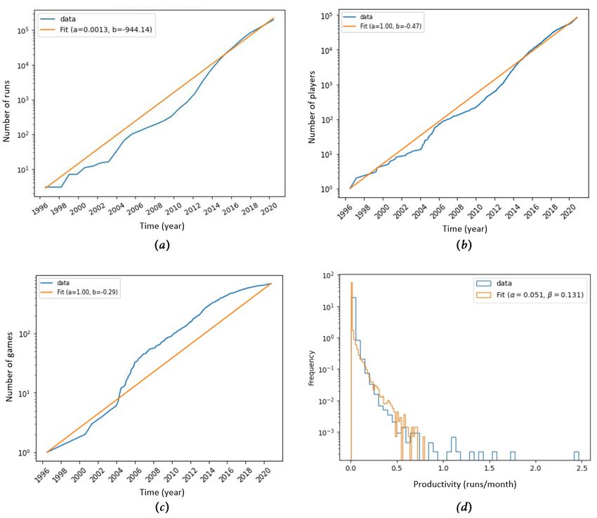
6Figure 1: (a) Growth in the number of speedruns over time. This growth is cumula-
tive since runs are not removed, and is parallel to that of the speedrunning community.
Empirical data (in blue) shows a quite exponential behaviour. An exponential fit (in
orange) was performed with growth rate µr = 0.507 1/year. (b) Growth in the number
of players over time and exponential fit (µp = 0.486 1/year). (c) Growth in the number
of games over time and exponential fit (µg = 0.270 1/year). (d ) Productivity frequency
distribution as number of runs per month. The empirical data (in blue) shows a decay in
which players submitting runs with higher frequency become rarer. This distribution has
been fitted (in orange) to a gamma process with parameters α = 0.051 and β = 0.131.
relating to periods of increased popularity or dissemination. Players and games also follow
an exponential description (Figure 1b and c, respectively) and were assumed to join the
community but not to leave it, since the mere fact of submitting a run reveals awareness
and represents an involvement in the community. Hence, the speedrunning community
grows by means of the following equation:
N (t) = N0 eµ(t−t0 ) , (1)
in which, according to the fit, time zero would be set at 1996, the initial population
7Figure 2: Rank-ordered distribution of players according to the number of runs submit-
ted: (a) simulated; (b) empirical (in blue); fit (in orange) assuming a DGBD (a = 0.480,
b = 0.528). Simulated results are congruent to those shown by the empirical data when
population growth and productivity are modelled using exponential dynamics.
according to speedrun.com would be N0 = 2 submissions, and the growth rate would
be µr = 0.507 1/year. Players and games have growth rates µp = 0.486 1/year and
µg = 0.270 1/year, respectively, and both an initial population N0 = 1. Growth rates can
be understood as the chance, for instance, that a player recruited another player in time,
or recruitments per time.
We define a player’s productivity π as the number of runs submitted per unit time by
a unique user. Results show how most users have less than 1 run per month, and that
productivity can be captured by an exponential/gamma distribution, as shown in Figure
1d ), in which it has been fitted to a gamma process:
β α α−1 −βπ
p(π) = π e , (2)
Γ(α)
where:
Z ∞
Γ(α) = π α−1 e−π dπ (3)
0
is the Gamma function. This marginal distribution has a shape parameter α and an
inverse-scaling parameter β, and has mean µ = αβ and variance σ 2 = αβ 2 . As can
be observed, player productivity can be described as a gamma process with parameters
α = 0.051 and β = 0.131, except for those few exceptional players who, in the shape of
apparently random bursts in the figure, submit runs with remarkably high frequency.
Then, a simulation was conducted in which, in each iteration, each player might recruit
another one to the community with chance µp . A certain productivity was assigned to
8Figure 3: Rank-ordered distribution of games according to their number of runs: em-
pirical (in blue); fit (in orange) assuming a DGBD (a = 0.473, b = 1.311).
each new runner following the aforementioned distribution. The simulation was stopped
when the empirical population size by November 2020 was reached (85,786 players), and
players were ranked according to their number of runs. As can be observed in Figure 2, the
results of the simulation resemble those shown by the empirical data, whose rank-ordered
distribution was also computed. In both cases, with both axes in logarithmic scale, the
absolute value of the slope of the curve increases as the rank number increases, in contrast
with the long asymptotic tail that characterizes power-law distributions. Moreover, the
empirical data also shows higher slopes (in absolute value) for those few players with the
highest number of runs.
In order to provide an analytical basis for the rank-ordered distributions obtained, they
were fitted to a so-called discrete generalized beta distribution (DGBD) [23]. This distri-
bution has the following equation:
(N + 1 − r)b
f (r) = A , (4)
ra
where N is the number of elements in the rank, r ∈ N is the position in the rank, A is
a normalization constant and parameters a and b are two fitting exponents. The balance
between a and b has its own meaning: a can be related to behaviours generating ordered
power-laws, whereas b is usually connected to disordered fluctuations in the distribution.
In other words, they represent the role of order and disorder shown by the rank. Many
systems from different fields have been observed to follow this distribution, such as the
frequency with which the codons appear in the genome of E. coli (a = 0.25, b = 0.50), the
number of collaborators a movie actor has worked with (a = 0.71, b = 0.61), the popular-
ity of programming languages or the occurrence of musical notes in different pieces [23, 24].
The results were fitted to a DGBD with A = 1, N = 85, 786, a = 0.480 and b = 0.528,
as can be observed in Figure 2b. In this case, a is quite similar to b, yet b > a, which
leads to think that disorder and fluctuation due to noise or external factors play a more
important role than the power-law-like behaviour.
9Figure 4: Score and date of all runs for different categories of the game New Super
Mario Bros. Wii: (a) Any%; (b) 100%. Each dot represents an individual run. Those
runs which represent new best scores are highlighted in orange. Using the best scores
only, a curve fit was performed in the shape of an exponential decay (see dashed curve
in red), with learning rates λ = 0.262 1/year (a) and λ = 1.033 1/year (b). Notice
that scores change between categories: whereas the 100% mode requires to complete all
what the game has to offer, the Any% mode is only focused on reaching the final credits,
allowing the player to skip an important part of the content. Hence, 100% takes more
time to complete and scores are larger, yet the learning rates have similar order. It is also
remarkable how Any% has many more submissions than 100%.
The same procedure was applied to the distribution of games, as can be observed in Figure
3. In such case, the DGBD fit has parameters A = 1, N = 693, a = 0.473 and b = 1.311.
b is also larger than a, even more than in the player scenario. It is remarkable how most
video games have at least 100 submissions.
2.2.2 An exponential decay model for performance improvement
The progress in individual categories was also assessed, evaluating how performance
(scores) changed over time, and an overall exponential decay in the learning was ob-
served, with significant improvements when the first speedruns are submitted, which tend
to stabilize towards a certain score as more runs are uploaded. This is coherent since,
unless new hitherto-unknown strategies are discovered, scores tend asymptotically to a
theoretical limit and improvements between new runs in time become smaller.
Even though each category for each video game has its own characteristics, all best scores
for each of them were fitted in the shape of an exponential curve:
SC (t) = (S0 − Sbest )e−λ(t−t0 ) + Sbest , (5)
where SC (t) represents the minimal score at time t for a given video game category C,
that is, the minimal time taken for the category to be completed at a certain date. S
always tends to improve. S0 is the first score registered and Sbest is the current record
10Figure 5: Probability density of the learning rates. The distribution has been fitted as
a Gamma process with parameters α = 0.00590 and β = 0.00581. However, the empirical
distribution shows various bursts for relatively large learning rates. It is coherent that
most runs do not show any improvement, and that high improvements are relatively
difficult to find, since they usually depend on chance or on discovering new strategies.
score (or, at least, the best score registered by the time the data set was downloaded); t0
(in years) is the time at which S0 was achieved and λ ≥ 0 is the so-called learning rate,
which tells about how relevant the improvements of the score are in relation with time.
An average learning rate hλi = 114.02 1/year, a maximal rate λmax = 8, 904.37 1/year
and a minimal rate λmin = 0 were found.
The exponential decay when fitting was assumed to tend asymptotically towards each best
score instead of towards zero, since video games have certain animations and unskippable
events which make them technically impossible to be completed in no time, that is, there
is a minimal compulsory time that will always work as a lower bound.
These curves only consider those runs which represent an improvement with respect to
the latest best score. The exponential fit was only applied to those categories with at least
two runs submitted providing the best score at their time (and whose date is known); if
there had been no improvement at all since S0 , which means that the initial score had
always been the best, the learning rate is zero (λmin ). The smallest nonzero learning rate
is λmin,nonzero = 0.067 1/year. The average learning rate for those categories in which
there has been at least one improvement is hλinonzero = 126.66 1/year.
In Figure 4, examples for 2 different categories for a specific video game are provided.
Improvements were also assessed in a local manner, by means of the determining the
learning rate between individual runs, that is, considering only two runs at a time. The
frequency distribution of local learning rates value was visualized, as shown in Figure 5.
The distribution was fitted to a gamma process, as done with productivity, in this case
with α = 0.00590 and β = 0.00581. Regardless of the fit, the empirical results show
additional peaks in the shape of bursts, revealing recurrent intervals in which players
manage to obtain remarkable improvements in a relatively short period of time.
113 Stage II. A minimal model for the structural growth
of the community
3.1 Methods
After studying how the speedrunning community evolves in terms of its growth in play-
ers, games and runs, obtaining a rank-ordered distribution for video game players and
determining the learning rates through time as a measure of performance, it is not known
whether these results are enough to provide information about the actual structure of the
community, that is, how players and games are connected with each other. This informa-
tion would allow to establish linkages between games and players and to identify possible
subcommunities within the whole structure.
Hence, we can apply network methods in order to determine the structure of the com-
munity and, furthermore, to try to replicate its structural growth through time. In the
following section, we propose a minimal model for the growth of the speedrunning commu-
nity in structural terms based on the information obtained in the previous stage. The aim
of this model is to compare its outcome with the actual network and to observe whether
the previous results per se are enough to predict such structure or not.
3.1.1 The model
The model considers three kinds of individuals: players, games and runs. Each player
p and game g are identified by a distinctive number, whereas runs r are tuples in the
shape (p, g). Both players and games are stored in vectors p and g and added to them
each time they are introduced to the community. Runs are stored in an adjacency list
R. Regarding the network, then, each player and game is a node and each run an edge
connecting nodes. As can be noticed, the graph is bipartite, since there are two types of
nodes and edges can connect only nodes of different kind. Hence, there are no self-edges
either. The graph is also undirected and unweighted.
Since we knew how many players, games and runs the community had at each point in
time, the growth of the network was simulated through iterations setting the number of
entities that there should be when each loop finished. Recall that the aim of the model
was to study whether or not there are structural properties of the community which can-
not be explained by its observable growth trends, and, thus, the growth in the number
of players, games and runs should evolve accordingly. Likewise, the rank-ordered distri-
butions for players and games according to their number of runs should also be reproduced.
The simulation starts with a single seed run, with the existence of one single player and
one single game. Then, iterations are performed adding as many players, games and runs
as required according to the actual data and the iteration step size. Each iteration has
three stages: (1) the allocation of new players to the community, (2) the allocation of
new games and (3) the allocation of new runs. It is possible that, especially during early
iterations, no new players nor games are introduced.
Two variants of the model were designed (which could actually be treated as independent
12models), each one with a different procedure to allocate runs to games and players. In
both scenarios, however, it was imposed that every player and game must always have at
least one run (recall that a user with no submissions is not a player).
In the first variant, each time a new player or game is introduced to the community, a
run is created linking the player to a random game or the new game to a random player
following certain probability functions. When both players and games are introduced, the
remaining runs for each iteration are created choosing random players and games each
time according to those functions.
The second approach considers an infectious model with duplication in which each new
player is introduced due to an elder player attracting the new individual to the commu-
nity, which implies that the new player does not play a random video game (as happens
in the previous scenario) but a game that the elder player has already played, as if the
new player became interested in a game that one of his friends, for instance, told him
or her about. Hence, allocated nodes tend to duplicate the behaviour and connections
of older ones, as already proposed in certain models for protein-protein interactions, and
in a manner related to the number of connections each node already has [25, 26, 27].
This approach aims to be more realistic, and random allocations like those from the first
scenario could still occur with a certain probability µ, which consider the possibility that
a player discovers and plays a new game on his or her own.
Both versions also consider the possibility that the network is not totally connected, with
the existence of multiple components, since it is possible that certain communities of
players are restricted to specific games and, thus, completely isolated from other regions
of the graph. In order to simulate this, it is possible that a new game and a new player
are created simultaneously and linked to one another so that such clusters could emerge:
they could either become eventually related to other regions of the network due to new
associations or links, or, on the contrary, remain isolated. Such allocations occur with
probability ρ.
No matter the way games and players are introduced, the simulation is designed so that
after each iteration the number of players, games and runs are the ones which have been
imposed by the actual data. Nevertheless, the chances for players or games to be chosen
are not equiprobable, and they are related to the number of submissions each player and
game has, which was determined in the previous stage of the study (see Figures 2 and 3).
To reproduce the rank-ordered distributions, two fitness functions were defined in order
to generate a probability distribution for players and runs when they have to be chosen
randomly. These functions give priority to those players and games which have more runs,
that is, those which are more recurrent in the adjacency list R. The default score for each
player and game when they are introduced is 1, but it can be increased according to these
score functions, one for players φp (n) and another for games φg (n), where n ∈ N stands
for the respective number of runs. These functions are only modified once a player or a
game have been chosen, so that their frequency is rewarded. These functions have been
defined via trial and error so that the best outcomes were obtained.
The fitness score for a given player i follows a linear description:
13φpi (ni ) = 1 + πkp (ni − 1), (6)
where ni is the number of runs player i has, π is a probability which determines whether
the fitness of a player should increase or not each time the player is chosen, and kp ∈ N
is the number of units the score should be increased each time.
Regarding games, we defined the following nonlinear function:
1 if ni < nθ1
φgi (ni ) = 1 + k1 if nθ1 ≤ ni ≤ nθ2 , (7)
1 + k1 + γk2 (ni − nθ2 ) if ni > nθ2
where γ is a probability analogous to π in the previous case, k1 and k2 are the number of
units to increase in each case, and nθ1 and nθ2 are thresholds. This function is defined in
a fashion that games with a number of runs above the thresholds become highly popular
with time, whereas those which do not overcome them do not reach such popularity and
remain with few players.
These functions could also be understood in physical terms: the number of runs associ-
ated to a player depends on his or her willingness and persistence. The more submissions
a player makes, the more chance a new run will be submitted by that person in com-
parison to others which have few. In the case of video games, whether a game is played
or not depends on its fame and popularity, so the fact that a function with thresholds
can be used could be related to a minimal influence required for the video game to succeed.
Recall that scores are updated each time one player or game is chosen. We define the
propensity pi of a player or game i as the probability of i to be chosen. pi is thus given
by the following equation:
φi
pi = P , (8)
j φj
where φi represents either φpi or φgi .
Once the simulation finishes, the resulting community always has as many players, games
and runs as the actual one, and their ranks describe the same trend, as can be observed
in Figure 6.
14Figure 6: (a) Empirical rank-ordered distribution of players according to their number of
runs with the DGBD fit. (b) Rank-ordered distribution obtained via simulation with the
following parameters: π = 0.9, kp = 2. (c) Empirical rank-ordered distribution of games
with the DGBD fit. (d ) Simulated rank-ordered distribution with parameters γ = 0.07,
k1 = 5, k2 = 2 and nθ1 = nθ2 = 100. This example is from a simulation using the approach
without duplication (ρ = 0.01).
3.1.2 Structural analysis of the community
After the simulation was executed, we generated graphs for the community using Python’s
library NetworkX 2.5, which allows to create many kinds of graphs for given sets of nodes
and edges. 50 simulations were performed, 25 for each approach, thus generating 50 differ-
ent graphs. Recall that, at the time the data set was downloaded and after the first stage
was performed, we obtained information about 203,009 runs for 693 games and 85,786
players. The network, hence, would have a total of 86,479 nodes connected by 203,009
edges. Considering the bipartite nature of the network, these characteristics imply a the-
oretical average degree hkp i = 2.37 for players (runs per player) and hkg i = 292.94 for
games (runs per game). It must be remarked, however, that repeated runs are considered
as a single edge in the network, reducing the actual degree.
As can be noticed, the size of the community is very large and, when it comes to network
15analysis, there were measures and operations which represented too much computational
load, such as obtaining a network projection so that only players were represented, for
instance. Even though a projection of the whole network was obtained, this new graph
had a number of edges in the order of 107 matching 85,786 nodes, which made further
computations such as centrality parameters inviable by conventional means.
Hence, considering the consistency in the exponential growth of players, games and runs,
the analysis was reduced to a simplified but parallel picture of the scenario, and we only
considered all submissions, members and games identified in the community up until 2013,
ignoring all later information. It has to be remarked that simulations required a different
parameter tuning for each specific approach. Such tuning was performed via trial an error.
For these simulations up to 2013, parameters used in the approach without duplication
were: π = 0.25, kp = 2, γ = 0.4, k1 = 2, k2 = 30, nθ1 = 10, nθ2 = 40 and ρ = 0.01; and, in
the design with duplication: π = 0.05, kp = 1, γ = 0.001, k1 = 10, k2 = 2, nθ1 = nθ2 = 1,
ρ = 0.4 and µ = 0.1.
Even though it was not so large, by 2013, the speedrunning community was already sig-
nificantly dense, with 1,606 runs for 205 games and 1,144 players. In this context, there
is an average degree hkp i = 1.404 for players and hkg i = 7.834 for games. Node degrees
are smaller than in the previous scenario since the total number of runs is significantly
smaller, yet the aim of the model was to identify structural properties in the network that
could not be predicted with the information already obtained, and such simplification still
represented a comparison between the actual structure and the potential of the proposed
model. Projections of the real and simulated networks could also be computed removing
games and having only players as nodes. Edges would then connect players sharing one or
more video games. Then, structural parameters about the networks and their projections
could be determined.
When it comes to node-specific properties, we could first identify node degree k, that is,
the number of connections each node in the network has. Computing the distribution of
degrees through the network would allow to know whether most of the nodes are highly
connected or only a few.
Second, centrality, which measures the influence of nodes in a network. In particular, we
determined three types of centrality. The first one is eigenvector centrality, which mea-
sures how much connected a node is in the network considering the connectivity of its
neighbours too, that is, it provides information about its influence in the network. The
higher the eigenvector centrality of a node, the more connections it will have with nodes
which have high eigenvector centrality themselves. The second one is closeness centrality,
which tells about the influence of nodes in a graph in terms of distances. It determines
the average farness with respect to all other nodes, and those with the shortest distances
are the ones with the highest values. The third one is betweenness centrality, which de-
termines how influential each node is when it comes to spreading information through
the network. Computing the unweighted shortest paths for all pairs of nodes, it allows to
identify nodes which might connect different clusters or modules, behaving as some sort
of bridge between them.
Regarding global properties of the network, we computed the following ones:
16First, modularity Q, which is a measure for the division of a graph in different groups or
subcommunities in which nodes are densely connected. It computes the number of edges
in a cluster minus the number of edges expected by chance in the cluster, and sums over
all clusters. A graph with high modularity possesses many of those clusters or modules
and has few connections between nodes from different modules. The software Gephi 0.9.2
offers a tool to compute the modularity of a graph. All other parameters were determined
via NetworkX.
Second, the global number of edges l. Even though it could be related to the number of
runs, it must be taken into account that repeated runs are only counted once. Further-
more, the number of edges generated in projections do not depend on runs but on the
relations between players through games. The average node degree hki for projections
was also obtained.
Third, global efficiency Eglobal , which is the average inverse of the shortest path lengths in
the network. Since it is possible that some clusters are disconnected from others (graphs
with multiple components), shortest path lengths and averages could possibly not be com-
puted due to infinite distances. Thus, global efficiency would turn infinite distances into
zero, allowing computations.
Finally, connectance C0 , which represents the ratio between the number of edges in a net-
work and the theoretical number of possible connections. Connectance does not consider
self-edges nor repeated links, and represents a constraint for the number of different graphs
possibly generated, since it is proven that diversity or variability decreases when C0 is too
high or too low and that it is maximal when C0 = 1/2 [28]. Connectance is thus defined as:
l
C0 = , (9)
n(n − 1)
where l is the number of edges in a graph and n the number of nodes. Notice that the
factor in the denominator M = n(n − 1) represents the total number of possible unique
connections removing self-edges.
Connectance could be measured both for bipartite graphs and projections. However, the
definition for each of them is necessarily different. It is not hard to observe that, in the
bipartite case, l represents the number of unique runs nr , that is, without counting re-
peated ones (games played by the same player more than once). Furthermore, since the
edges of the bipartite graphs link players to video games, the number of possible edges is
M = np × ng , where np and ng are the number of players and games, respectively. On the
other hand, even though projections have nodes of the same kind (players), the number
of links l results from the connections between players through games, which depends on
the intrinsic structural properties of the network.
Hence, the connectance for the player-game bipartite networks turns out to be:
17nr
C0 = , (10)
np ng
and the one for projections with only players is:
l
C0 = . (11)
np (np − 1)
Finally, the projections with only players were visualized using Gephi 0.9.2.
3.2 Results
3.2.1 Properties of the community as a network
As aforementioned, the algorithm was executed for a total of 50 realizations, 25 for each
approach (with duplication and without), generating 50 different graphs. A graph for the
actual network was also generated. First, we determined the node degree distribution for
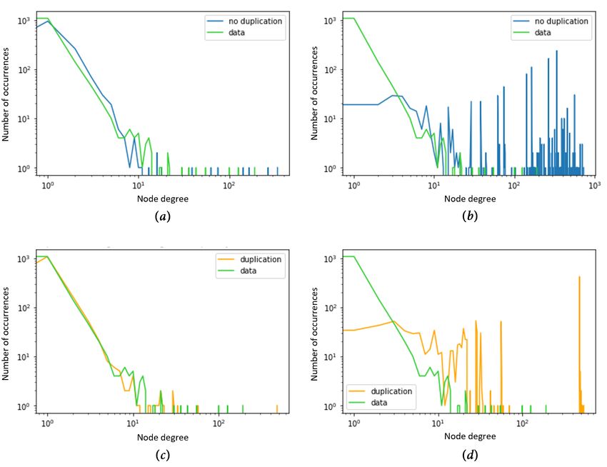
each graph, and compared it with the real data. In Figure 7a and c, a comparison of the
degree distribution from the actual bipartite graph with that from the simulations (as an
average) is shown. Since the degree, that is, the number of runs per player and per game,
and its distribution have to do with the rank-ordered distribution of players and games,
which was preserved in the simulation, it is logical that both cases follow the same dis-
tribution of degree occurrence: only a few players have a large number of runs, whereas
the majority has less than 10. Figure 7b and d show the same information but from
projections. It can be observed how most of the players in the actual community have
a very low degree (they are not much connected with each other), whereas simulations
show distributions remarkably different, with high occurrences for relatively large degrees,
implying that the model connects players through games more than in reality. The cases
with duplication (Figure 7d ), however, show better results than those without (Figure
7b): with a duplication model, players tend to play the same games which people who
introduce them into the community play, thus making it difficult for players to connect
with others who play different games.
We also computed the average node degree as a global property of the projections. The
projection of the actual community has average degree hkireal = 31.813. As can be ob-
served in Figure 8, both approaches tend to show larger values than hkireal , as can be
expected from Figure 7. This reinforces the observation that, even though simulations
follow the growth properties found in the first stage of the study, they establish more
connections between players than in real life. If an individual plays a large number of
games, it will certainly be connected to many more players than if the individual played
a few or only one. Even if a game has a massive amount of popularity, players will still
be more likely to be connected to others if they play multiple games. This might explain
why when allocations were performed only according to the fitness functions without du-
18Figure 7: Node degree average occurrence distribution among the 25 networks gener-
ated in each approach (in blue: no duplication; in orange: duplication) and the actual
community (in green). (a) and (c) show distributions for the respective bipartite graphs,
whereas (b) and (d ) show the ones for projections with only players. Since all graphs have
the same number of nodes, this figure takes the sum of the occurrence of each degree in
each of the 25 graphs for each case and divides it by the number of graphs.
plication, larger degrees were reached.
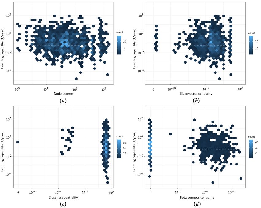
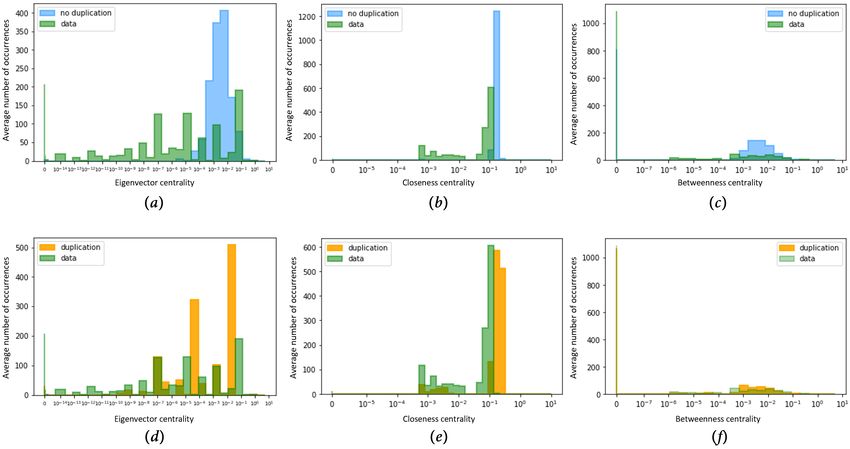
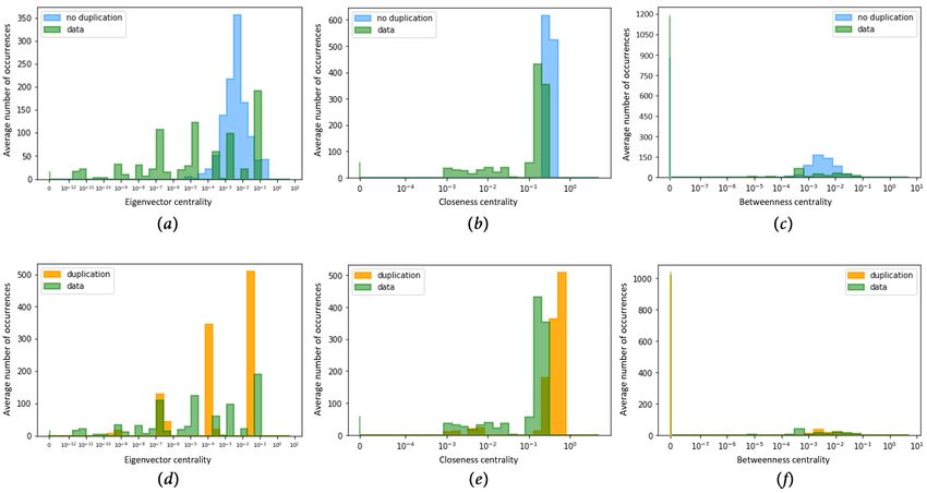
We then computed centrality parameters, and their distribution can be observed in Fig-
ure 9 and Figure 10 regarding the bipartite graphs and their projections, respectively,
as an average of the occurrences among each of the 25 simulations conducted with each
approach. In the figures, information about both kinds of simulations and about the real
graph is included. Regarding eigenvector centrality, it is observed how, both in the case of
bipartite graphs and projections, the actual network has low values with more frequency
than simulations, which reveals that simulations were not able to consider the fact that
only a few nodes have special influence in the network whereas most are not prominent.
Even though simulations with the duplication model managed to obtain lower values,
they are still too high and their distribution is closer to those without duplication than
to the actual one. Closeness centrality and betweenness centrality, on the other hand,
show more accurate results. In the case of closeness centrality, especially in simulations
with the duplication model (Figure 9e and Figure 10e), distributions are similar to the
original, yet many nodes still have too high values. Real data shows a higher number of
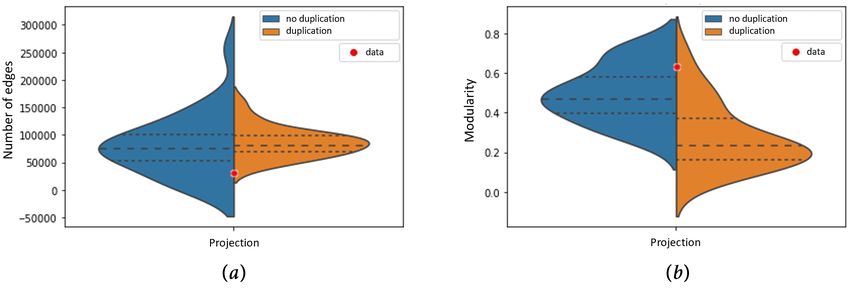
19Figure 8: Average node degree among the 25 networks generated in projections (blue:
no duplication; orange: duplication model). The real average degree is depicted with a
red dot on the vertical axis of the violin plot. It can be observed how simulations without
a duplication model lead to a wider range of values.
occurrences in relatively large values of closeness centrality: players could be clustered in
dense modules which could be connected by remarkably short paths (a very small number
of players behaving as bridges between modules). Regarding betweenness centrality, in
Figure 9c and f and Figure 10c and f, it can be observed how, even though simulations
without duplication show high values with higher frequency than the original graph and
those with duplication, most nodes have their betweenness centrality equal to zero in all
scenarios: not many nodes play an important role in connecting modules or substruc-
tures in the networks. It should also be considered that graphs can have more than one
component, with two or more unconnected structures (which could also explain the high
occurrence of nodes with zero eigenvector centrality in the real bipartite network, as ob-
served in Figure 9a or d ). Those few nodes with high betweenness centrality, on the
other hand, lie around the same interval in all cases. Regarding centrality in general, it
could be thought that, the higher the connection between players (as observed with node
degrees), the more frequent influential players are (and games too in the bipartite case),
leading to a higher frequency of high centrality values in simulations with no duplication,
in which individuals play different games each time allocated randomly and, thus, players
are connected with more players and from different areas in the network.
When it comes to the global efficiency, it can be observed in Figure 11 how in all simu-
lations for both kinds of graphs (bipartite and projections) values are remarkably larger
than real efficiencies (0.083 for the bipartite case and 0.197 for the projection). Recall
that global efficiency is the average inverse of the shortest path lengths in a graph: higher
efficiencies imply that distances between nodes are smaller. Hence, in simulations, given
the higher connection between individuals playing different games and, in projections,
the higher number of connections between players, individuals are globally closer to one
another than in the real community. This higher number of connections can be observed
in Figure 12a, in which the number of edges in projections is shown. Notice, however, that
they can be determined as the sum of all degrees divided by 2, so they have a meaning
similar to average node degrees. It can be highlighted again how most of the simulated
graphs create too many connections between players in comparison to the actual network
(whose number of connections is lreal = 36, 394 edges).
20You can also read