MP3: A Unified Model to Map, Perceive, Predict and Plan
←
→
Page content transcription
If your browser does not render page correctly, please read the page content below

MP3: A Unified Model to Map, Perceive, Predict and Plan

                                                                  Sergio Casas*,1,2 , Abbas Sadat ∗,1 , Raquel Urtasun1,2
                                                                          Uber ATG1 , University of Toronto2
                                                        {sergio, urtasun}@cs.toronto.edu, abbas.sadat@gmail.com
arXiv:2101.06806v1 [cs.RO] 18 Jan 2021

                                                                      Abstract                                              Driving with an HD map              Mapless driving

                                             High-definition maps (HD maps) are a key component of                                                            “Turn Right”
                                         most modern self-driving systems due to their valuable se-
                                         mantic and geometric information. Unfortunately, building
                                         HD maps has proven hard to scale due to their cost as well
                                         as the requirements they impose in the localization system
                                         that has to work everywhere with centimeter-level accuracy.
                                         Being able to drive without an HD map would be very bene-
                                         ficial to scale self-driving solutions as well as to increase the
                                                                                                                        Figure 1: Left: a localization error makes the SDV follow
                                         failure tolerance of existing ones (e.g., if localization fails or
                                                                                                                        a wrong route when using an HD map, driving into traffic.
                                         the map is not up-to-date). Towards this goal, we propose
                                                                                                                        Right: mapless driving can interpret the scene from sensors
                                         MP3, an end-to-end approach to mapless1 driving where
                                                                                                                        and achieve a safe plan that follows a high-level command.
                                         the input is raw sensor data and a high-level command (e.g.,
                                         turn left at the intersection). MP3 predicts intermediate
                                         representations in the form of an online map and the current                   the ego-vehicle that adhere to the traffic rules. In addition,
                                         and future state of dynamic agents, and exploits them in a                     progressing towards a specific goal is much simpler when
                                         novel neural motion planner to make interpretable decisions                    the desired route is defined as a sequence of lanes to traverse.
                                         taking into account uncertainty. We show that our approach                         Unfortunately, building HD maps has proven hard to
                                         is significantly safer, more comfortable, and can follow com-                  scale due to the complexity and cost of generating the maps
                                         mands better than the baselines in challenging long-term                       and maintaining them. Furthermore, the heavy reliance on
                                         closed-loop simulations, as well as when compared to an                        HD maps introduces very demanding requirements for the
                                         expert driver in a large-scale real-world dataset.                             localization system, which needs to work at all times with
                                                                                                                        centimeter-level accuracy or else unsafe situations like Fig. 1
                                                                                                                        (left) might arise. This motivates the development of mapless
                                         1. Introduction                                                                technology, which can serve as the fail-safe in the case of
                                            Most modern self-driving stacks require up-to-date high-                    localization failures or outdated maps, and potentially unlock
                                         definition (HD) maps that contain rich semantic information                    self-driving at scale at a much lower cost.
                                         necessary for driving such as the topology and location of                         Self-driving without HD maps is a very challenging task.
                                         the lanes, crosswalks, traffic lights, intersections as well as                Perception can no longer rely on the prior that is more likely
                                         the traffic rules for each lane (e.g., unprotected left, right turn            to find vehicles on the road and pedestrians on the sidewalk.
                                         on red, maximum speed). These maps are a great source of                       Motion forecasting of dynamic objects becomes even more
                                         knowledge that simplify the perception and motion forecast-                    challenging without having access to the lanes that vehicles
                                         ing tasks, as the online inference process has to mainly focus                 typically follow or the location of crosswalks for pedestrians.
                                         on dynamic objects (e.g., vehicles, pedestrians, cyclists).                    Most importantly, the search space to plan a safe maneuver
                                         Furthermore, the use of HD maps significantly increases the                    for the SDV goes from narrow envelopes around the lane cen-
                                         safety of motion planning as knowing the lane topology and                     ter lines [1, 45, 46, 50] to the full set of dynamically feasible
                                         geometry eases the generation of potential trajectories for                    trajectories as depicted in Fig. 1 (right). Moreover, without
                                                                                                                        a well-defined route as a series of lanes to follow, the goal
                                            * Denotes equal contribution
                                            1 We note that by mapless we  mean without HD maps. A coarse road
                                                                                                                        that the SDV is trying to reach needs to be abstracted into
                                         network like the ones available in off-the-shelf services such as Google       high-level behaviors such as going straight at an intersec-
                                         Maps or OpenStreetMap is assumed available for routing towards the goal.       tion, turning left or turning right [11], which require taking

                                                                                                                    1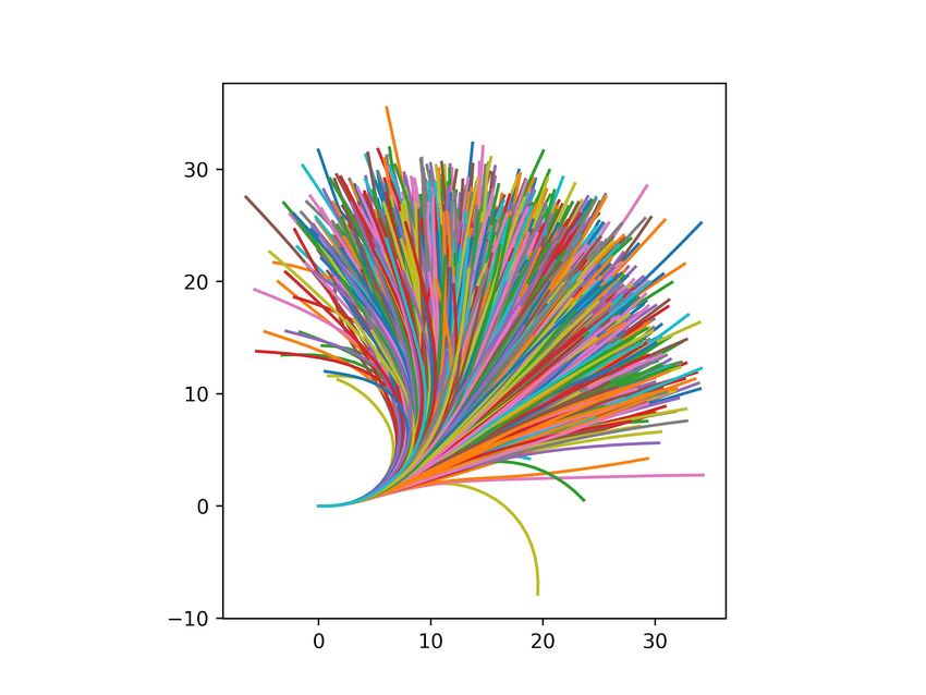
different actions depending of the context of the scene.                 a human-in-the-loop. For these reasons, such approaches
    Most mapless approaches [5, 11, 19, 37, 39], focus on im-            are not suitable for mapless driving. As a consequence, pre-
itating the controls of an expert driver (e.g., steering and             dicting map elements online has recently been proposed.
acceleration), without providing intermediate interpretable              In [16, 18] a network is presented to directly predict the 3D
representations that can help explain the self-driving vehicle           layout of lanes in a traffic scene from a single image. Con-
decisions. Interpretability is of key importance in a safety-            versely to the methods above, [2] argues that accurate image
critical system particularly if a bad event was to happen.               estimates do not translate to precise 3D lane boundaries,
Moreover, the absence of a mechanism to inject structure                 which are the input required by modern motion planning
and prior knowledge makes these methods very brittle to                  algorithms. To tackle this, LiDAR and camera are used to
distributional shift [44]. While methods that perform online             predict estimates of ground height and lanes directly in 3D
mapping to obtain lane boundaries or lane center lines have              space. Alternatively, [21] proposes a hierarchical recurrent
been proposed [2, 16, 18, 21, 37], they either are overly sim-           neural network for extraction of structured lane boundaries
plistic (e.g., assume lanes are close to parallel to the direction       from LIDAR sweeps. Notably, all the works above are
of travel), have only been demonstrated in highway scenar-               geared toward highway traffic scenes and involve discrete
ios which are much simpler than city driving, have not been              decisions that could be unsafe when driving as they lose
shown to work when coupled with any existing planner, or                 valuable uncertainty information. Contrary to these methods,
involve information loss through discrete decisions such as              we leverage dense representations of the map that do not in-
confidence thresholding to output the candidate lanes. The               volve information loss and are suitable for use in the motion
latter is safety-critical as a lane can be completely missed             planner as interpretable cost functions.
in the worst case, and it makes it difficult to incorporate
uncertainty about the static environment in motion planning,             Perception and Prediction: Most previous works per-
which is importance to reduce risk.                                      form object detection [15, 25, 34, 53, 57] and actor-based
    To address these challenges, we propose an end-to-end                prediction to reason about the current and future state of
approach to mapless driving that is interpretable, does not              a driving scene. As there are multiple possible futures,
incur any information loss, and reasons about uncertainty in             these methods either generate a fixed set of trajectories
the intermediate representations. In particular, we propose              [6, 8–10, 26, 28, 30, 36, 56], draw samples to characterize
a set of probabilistic spatial layers to model the static and            the distribution [7, 41, 47] or predict temporal occupancy
dynamic parts of the environment. The static environment is              maps [23, 27, 43]. However, these pipelines can be unsafe
subsumed in a planning-centric online map which captures                 since the detection stage involves confidence thresholding
information about which areas are drivable and which ones                and non-maximum suppression which can remove unconfi-
are reachable given traffic rules. The dynamic actors are cap-           dent detections of real objects. In robotics, occupancy grids
tured in a novel occupancy flow that provides occupancy and              at the scene-level (in contrast to actor-level) have been a
velocity estimates over time. The motion planning module                 popular representation of free space. Different from the
then leverages these representations without any postpro-                methods above, [13, 48] estimate occupancy probability of
cessing. It utilizes observational data to retrieve dynamically          each grid-cell independently using range sensor data. More
feasible trajectories, predicts a spatial mask over the map to           recently, [20] directly predicts an occupancy grid to replace
estimate the route given an abstract goal, and leverages the             object detection, but it does not predict how the scene might
online map and occupancy flow directly as cost functions for             evolve in the future. [45] improves over such representation
explainable, safe plans. We showcase that our approach is                by adding semantics as well as future predictions. However,
significantly safer, more comfortable, and can follow com-               there is no way to extract velocity from the scene occupancy,
mands better than a wide variety of baselines in challenging             which is important for motion planning. While [51] con-
closed-loop simulations, as well as when compared to an                  siders a dense motion field, their parameterization cannot
expert driver in a large-scale real-world dataset.                       capture multi-modal behaviors. We follow the philosophy
                                                                         of [13,20,45,48,51] in predicting scene-level representations,
2. Related Work                                                          but propose an improved occupancy flow parameterization
   We cover previous works on online mapping, perception                 that can model multi-modal behavior and provides a consis-
and prediction, and motion planning, particularly analyzing              tent temporal motion field.
their fitness to the downstream task of end-to-end driving.
                                                                         Motion Planning: There is a vast literature on end-to-end
Online Mapping: While there are many offline mapping                     approaches for self-driving. The pioneering work of [39]
approaches [4, 22, 33], these rely on satellite imagery or               proposes to use a single neural network that directly outputs
multiple passes through the same scene with a data collec-               a driving control command. Subsequent to the success of
tion vehicle to gather dense information, and often involve              deep learning, direct control based methods have advanced

                                                                     2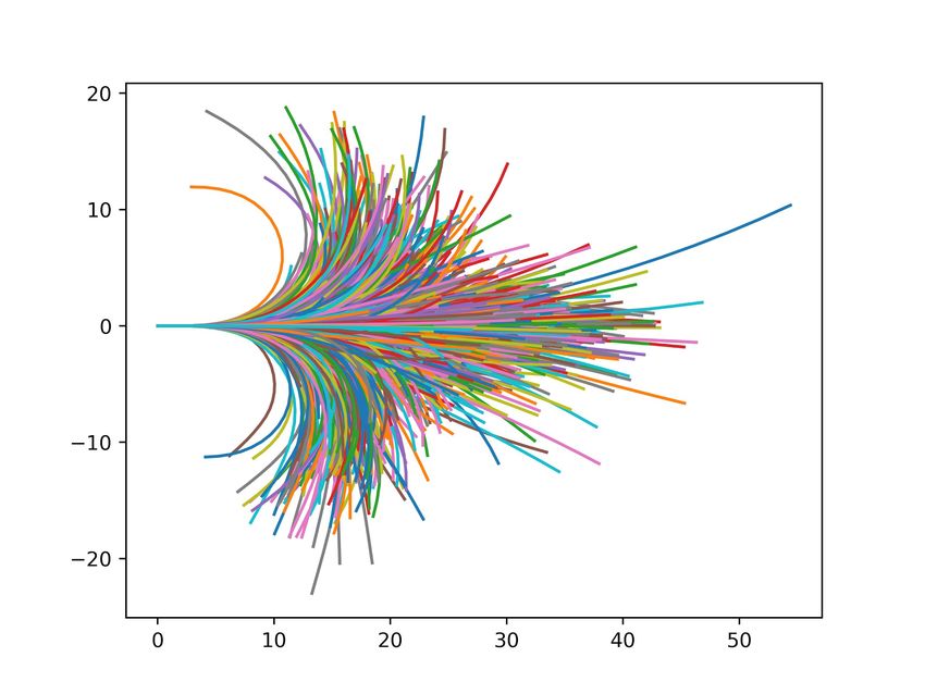
Inputs                           Scene Representations                      Motion Planning

                                         Mapping       Online map               Retrieval-based
     Voxelized LiDAR      Backbone                                                                                   SDV
                           Network                                             Trajectory sampler
                                                                                                                  Trajectory
                                                                                                    Costing

                                       Perception &
                                        Prediction Dynamic state
     High-level Goal                                                              Routing

     “Keep Straight”

Figure 2: MP3 predicts probabilistic scene representations that are leveraged in motion planning as interpretable cost functions

with deeper networks, richer sensors, and scalable learning          interpretable representations, and show how they can be ex-
methods [5, 11, 24, 35]. Although simple and general, such           ploited to plan maneuvers that are safe, comfortable, and
methods of directly generating control command from sensor           explainable. An overview of our model can be seen in Fig. 2
data may have stability and robustness issues [12]. More re-
cently, cost map-based approaches have been shown to adapt           3.1. Extracting Geometric and Semantic Features
better to challenging environments, which recover a trajec-             Our model exploits a history of LiDAR point clouds to
tory by looking for local minima on the cost map. The cost           extract rich geometric and semantic features from the scene
map may be parameterized as a simple linear combination              over time. Following [30], we voxelize Tp =10 past LiDAR
of hand crafted costs [14, 46], or in a general non-parametric       point clouds in bird’s eye view (BEV), equivalent to 1 second
form [55]. To bridge the gap between interpretability and ex-        of history, with a spatial resolution of a = 0.2 meters/voxel.
pressivity, [45] proposed a model that leverages supervision         We exploit odometry to compensate for the SDV motion,
to learn an interpretable nonparametric occupancy that can           thus voxelizing all point clouds in a common coordinate
be directly used in motion planner, with hand-crafted sub-           frame. Our region of interest is W =140m long (70m front
costs. In contrast to all methods above which rely on an HD          and behind of the SDV), H=80m wide (40 to each side of the
map, [31] proposes to output a navigation cost map without           SDV), and Z=5m tall. Following [9], we concatenate height
localization under a weakly supervised learning environment.         and time along the channel dimension to avoid using 3D
This work, however, does not explicitly predict the static and       convolutions or a recurrent model, thus saving memory and
dynamic objects and hence lacks safety and interpretability.         computation. The result is a 3D tensor of size ( H   W Z
                                                                                                                      a , a , a ·Tp ),
Similarly, [3] improves sampling in complex driving envi-            which is the input to our backbone network. This network
ronments without the consideration of dynamic objects, and           combines ideas from [9, 53] to extract geometric, semantic
is only demonstrated in simplistic static scenarios. In con-         and motion information about the scene. More details can
trast, our autonomy model leverages retrieval from expert            be found in the appendix.
demonstrations to achieve an efficient trajectory sampler that
does not rely on the map, predicts a spatial route based on
                                                                     3.2. Interpretable Scene Representations
the probabilistic map predictions and a high-level driving              Human drivers are able to successfully navigate complex
command, and stays safe by exploiting an interpretable dy-           road topologies with high-density of traffic by exploiting
namic occupancy field as a summary of the scene free space           their prior knowledge about traffic rules and social behavior
and motion.                                                          such as the fact that vehicles should drive on the road, close
                                                                     to a lane centerline, in the direction of traffic and should not
3. Interpretable Mapless Driving                                     collide with other actors. Since we would like to incorporate
   In this section, we introduce our end-to-end approach to          such prior knowledge into the decisions of the SDV, and
self-driving that operates directly on raw sensor data. Im-          these to be explainable through interpretable concepts, it
portantly, our model produces intermediate representations           is important to predict intelligible representations of the
that are designed for safe planning, decision-making and             static environment, which we refer here as an online map,
interpretability. Our interpretable representations estimate         as well as the dynamic objects position and velocity into the
the current and future state of the world around the SDV,            future, captured in our dynamic occupancy field. We refer
including the unknown map as well as the current and future          the reader to Fig.3 for an example of these representations.
location and velocity of dynamic objects. In the remainder           Since the predicted online map and dynamic occupancy field
of this section, we first describe our backbone network that         are not going to be perfect due to limitations in the sensors,
extracts meaningful geometric and semantic features from             occlusions and the model, it is important to reason about
the raw sensor data. We then introduce our intermediate              uncertainty to assess the risk of each possible decision the

                                                                 3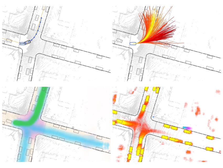
t=0             t=1                 t=2

                                                                         Occupancy
                                                                                            Flow                Flow

           Drivable area                     Intersections

                                                                         Motion
 Reachable Distance Transform             Reachable Angle                Figure 4: The motion field warps the occupancy over time.
                                                                         Transparency denotes probability. Color differences the pre-
                                                                         dicted layers by the network and the future occupancy. We
                                                                         depict the particular case of unimodal motion (K = 1).

            Occupancy                  Temporal Motion Field             methods contain unsafe discrete decisions such as confi-
Figure 3: Interpretable Scene representations. For occu-                 dence thresholding and non-maximum suppression (NMS)
pancy and motion, we visualize all time steps and classes in             that can eliminate low-confidence predictions of true objects
the same image to save space, differentiating with colors.               resulting in unsafe situations. [45] proposed a probabilis-
                                                                         tic way to measure the likelihood of a collision for a given
SDV might take. Next, we first describe the semantics in our             SDV maneuver by exploiting a non-parametric spatial repre-
interpretable representation of the world, and then introduce            sentation of the world. This computation is agnostic to the
our probabilistic model.                                                 number of objects. However, this representation does not
                                                                         provide velocity estimates, and thus it is not amenable to
Online map representation: In order to drive safely it is                car-following behaviors and speed-dependent safety buffer
useful to reason the following elements in BEV:                          reasoning. Moreover, the decision making algorithm cannot
                                                                         properly reason about interactions, since for a given future
- Drivable area: Road surface (or pavement) where vehicles
                                                                         occupancy its origin cannot be traced back.
  are allowed to drive, bounded by the curb.
                                                                             In contrast, in this paper we propose an occupancy flow
- Reachable lanes: Lane center lines (or motion paths) are               parameterized by the occupancy of the dynamic objects at
  defined as the canonical paths vehicles travel on, typically           the current state of the world and a temporal motion field into
  in the middle of 2 lane markers. We define the reach-                  the future that describes how objects move (and in turn their
  able lanes as the subset of motion paths the SDV can get               future occupancies), both discretized into a spatial grid on
  to without breaking any traffic rules. When planning a                 BEV with a resolution of 0.4 m/pixel, as depicted in Fig. 4:
  trajectory, we would like the SDV to stay close to these
                                                                         - Initial Occupancy: a BEV grid cell is active (occupied)
  reachable lanes and drive aligned to their direction. Thus,
                                                                           if its center falls in the interior of a polygon given by an
  for each pixel in the ground plane we predict the unsigned
                                                                           object shape and its current pose.
  distance to the closest reachable lane centerline, truncated
  at 10 meters, as well as the angle of the closest reachable            - Temporal Motion Field: defined for the occupied pixels
  lane centerline segment.                                                 at a particular time into the future. Each occupied pixel
- Intersection: Drivable area portion where traffic is con-                motion is represented with a 2D BEV velocity vector (in
  trolled via traffic lights or traffic signs. Reasoning about             m/s). We discretize this motion field into T = 11 time
  this is important to handle stop/yield signs and traffic lights.         steps into the future (up to 5s, every 0.5s).
  For instance, if a traffic light is red, we should wait to en-            Since the SDV behavior should be adaptive to objects
  ter the intersection. Following [42], we assume a separate             from different categories (e.g., extra caution is desired
  camera-based perception system detects the traffic lights              around vulnerable road users such as pedestrians and bi-
  and recognizes their state as this is not our focus.                   cyclists), we consider vehicles, pedestrians and bikes as
                                                                         separate classes, each with their own occupancy flow.
Dynamic occupancy field: Another critical aspect to
achieve safe self-driving is to understand which space is                Probabilistic Model: We would like to reason about un-
occupied by dynamic objects and how do these move over                   certainty in our online map and dynamic occupancy field.
time. Many accurate LiDAR-based object detectors have                    Towards this goal, we model each semantic channel of the
been proposed [25, 34, 53, 57] to localize dynamic obstacles             online map M as a collection of independent variables per
followed by a motion forecasting stage [7, 10, 30, 41, 47] to            BEV grid cell. This assumption makes the model very sim-
predict the future state of each object. However, all these              ple and efficient. To simplify the notation, we use the letter i

                                                                     4
to indicate a spatial index on the grid instead of two indices                 a safe headway to the occupied area in front of the SDV.
(row, column) from now on. We model each BEV grid cell                         The probabilistic layers in our online map are used in the
in the drivable area and intersections channels as Bernoulli                   scoring function to ensure the SDV is driving on the drivable
random variables, MA              I                                            area, close to the lane center and in the right direction, being
                        i and Mi respectively, as we consider
a grid cell is either part these elements or not. We model the                 cautious in uncertain regions, and driving towards the goal
truncated distance transform to the reachable lanes centerline                 specified by the input high-level command. The planner
                                                                               evaluates all the sampled trajectories in parallel and selects
MD  i as a Laplacian, which we empirically found to yield                      the trajectory with the minimum cost:
more accurate results than a Gaussian, and the direction of
the closest lane centerline in the reachable lanes Mθi as a                                   τ ∗ = argmin f (τ, M, O, K, V; w)
                                                                                                    τ ∈T (x0 )
Von Mises distribution since it has support between [π, π].
    We model the occupancy of dynamic objects Oc for                            with f the scoring function, w the learnable parameters
each class c ∈ {vehicle, pedestrian, bicyclist} as a collec-                   of our models, M the map layers, O, K, V the occupancy
                                        c                                      and motion mode-probability and vector layers respectively,
tion of Bernoulli random variables Ot,i   , one for each spatio-
temporal index t, i. Since an agent future behavior is highly                  and T (x0 ) represents the possible trajectories which are
uncertain and multi-modal (e.g., a vehicle going straight                      generated conditioned on the current state of the SDV x0 .
vs. turning right), we model the motion for each class at
each spatio-temporal location as a categorical distribution                    3.3.1   Trajectory Sampling
  c                                       c
Kt,i  over K BEV motion vectors {Vt,i,k        : k ∈ 1 . . . K}.
Here, each motion vector is parameterized by the continu-                      The lane centers and topology are strong priors to construct
ous velocity in the x and y directions in BEV. To compute                      the potential trajectories to be executed by the SDV. When an
the probability of future occupancy under our probabilistic                    HD map is available, the lane geometry can be exploited to
model, we first define the probability of occupancy flowing                    guide the trajectory sampling process. A popular approach,
from location i1 to location i2 between two consecutive time                   for example, is to sample trajectories in Frenet-frame of the
steps t and t + 1 as follows:                                                  goal lane-center, limiting the samples to motions that do not
   c
p(F(t,i               )=
                           X      c
                               p(Ot,i       c
                                        )p(Kt,i          c
                                                  = k)p(Vt,i      = i2 )       deviate much from the desired lane [1, 45, 46, 50]. However,
        1 )→(t+1,i2 )                 1         1            1 ,k
                           k                                                   in mapless driving we need to take a different approach as the
                                                                               HD map is not available. We thus use retrieval from a large-
 where p(Vt,i1 ,k = i2 ) distributes the mass locally and is                   scale dataset of real trajectories. This approach provides a
determined via bilinear interpolation if i2 is among the 4                     large set of trajectories from expert demonstrations while
nearest grid cells to the head of the continuous motion vec-
                                                                               avoiding random sampling or arbitrary choices of accelera-
tor, and 0 for all other cells, as depicted in Fig. 4. With
this definition, we can easily calculate the future occupancy                  tion/steering profiles [36, 55]. We create a dataset of expert
iteratively, starting from the occupancy predictions at t = 0.                 demonstrations by binning based on the SDV initial state,
This parameterization ensures consistency by definition be-                    clustering the trajectories of each bin, and using the cluster
tween future motion and future occupancy, and provides an                      prototypes for efficiency. During online motion planning, we
efficient way to query how does some particular initial occu-                  retrieve the trajectories of the bin specified by (vx , ax , κx )
pancy evolve over time, which will be used for interaction                     with x the current state of the SDV. However, the retrieved
and right-of-way reasoning in our motion planner. Specif-                      trajectories may have marginally different initial velocity and
ically, to get the occupancy that flows into cell i at time                    steering angle than the SDV. Hence, instead of directly using
t + 1 from all cells j at time t, we can simply compute the                    those trajectories, we use the acceleration and steering rate
probability that no occupancy flow event occurs, and take its                  profiles, (a, κ̇)t , t = 0, ..., T , to rollout a bicycle model [38]
complement
                               Y
                                                                               starting from the initial SDV state. This process generates
             c                             c
                                                                               trajectories with continuous velocity and steering. This is

          p(Ot+1,i )=1−             1 − p(F(t,j)→(t+1,i) )
                                j                                              in contrast to the simplistic approach of, e.g., [37] where a
                                                                               fixed set of template trajectories is used, ignoring the initial
We point the reader to the appendix for further details on the
mapping and perception and prediction network architecture.                    state of SDV.

3.3. Motion Planning                                                           3.3.2   Route Prediction
   The goal of the motion planner is to generate trajectories                  When HD maps are available, the input route is typically
that are safe, comfortable and progressing towards the goal.
We design a sample-based motion-planner in which a set                         given in the form of a sequence of lanes that the SDV should
of kinematically-feasible trajectories are generated and then                  follow. In mapless driving however, this is not possible. In-
evaluated using a learned scoring function. The scoring                        stead, we assume we are given a driving command as a tuple
function utilizes the probabilistic dynamic occupancy field                    c = (a, d), where a ∈ {keep lane, turn left, turn right} is a
to encode the safety of the possible maneuvers encouraging                     discrete high-level action, and d an an approximate longitu-
cautious behaviors that avoid occupied regions, and maintain                   dinal distance to the action. This information is similar to

                                                                           5
what an off-the-shelf GPS-based navigation system provides            where m(x) is the set of BEV grid-cells that overlap with
to human drivers. To simulate GPS errors, we randomly                SDV at trajectory point x. Similarly, the SDV needs to avoid
sample noise from a zero-mean Gaussian with 5m standard              junctions with red-traffic lights. Hence. we use the predicted
deviation. We model the route as a collection of Bernoulli           junction probability map MJ to penalize maneuvers that
random variables, one for each grid cell in BEV. Given the           violate red-traffic light, similar to the routing cost.
driving command c and the predicted map M, a routing
network predicts a dense probability map R in BEV. The               Safety: The predicted occupancy layers and motion pre-
routing network is composed of 3 CNNs that act like a switch         dictions are used to score the trajectory samples with respect
for the possible high-level actions a. Note that only the one        to safety. We penalize trajectories where the SDV overlaps
corresponding to the given driving command will be run               occupied regions. For each trajectory point, we use the BEV
at inference. Together with the predicted map layers, we             grid-cell with maximum probability among all the grid-cells
”rasterize” the longitudinal distance d to the action as an          that overlap with SDV polygon and use this probability di-
additional channel (i.e., repeated spatially), and leverage          rectly as collision cost. The max operator ensures that the
CoordConv [29] to break the translation invariance of CNNs.          worst-case occupancy is considered over the region SDV
                                                                     occupies.
                                                                        The above objective promotes trajectories that do not
3.3.3   Trajectory Scoring                                           overlap with occupied regions. However, the SDV needs
                                                                     to also maintain a safe distance from objects that are in
We use a linear combination of the following cost functions          the direction of SDV motion. This headway distance is
to score the sampled trajectories. More detailed explanations        a function of the relative speed of the SDV wrt the other
about the individual costs can be found in the appendix.             objects. To compute this cost for each trajectory point x, we
                                                                     retrieve all the BEV grid-cells in front of the SDV at x and
Routing and Driving on Roads: In order to encourage
                                                                     measure the violation of safety distance if the object at each
the SDV to perform the high-level command, we use a scor-
ing function that encourages trajectories that travel a larger       of those grid-cells stops with hard deceleration, and SDV
distance in regions with high probability in R. We use the           with state xt reacts with a comfortable deceleration.
following score function:
                                                                     Comfort: We also penalize jerk, lateral acceleration, cur-
                fr (τ, R) = −m(τ ) min Ri                            vature and its rate of change to promote comfortable driving.
                                    i∈m(τ )

 where m(τ ) is the BEV grid-cells that overlap with SDV
polygon in trajectory τ . This score function makes sure the         3.4. Learning
SDV stays on the route and is only rewarded when moving                  We optimize our driving model in two stages. We first
within the route. We introduce an additional cost-to-go that         train the online map, dynamic occupancy field, and routing.
considers the predicted route beyond the planning horizon.           Once these are converged, in a second stage, we keep these
This is important when there is a turn at the end of the hori-       parts frozen and train the planner weights for the linear
zon and the SDV velocity is high. Specifically, we compute           combination of scoring functions. We found this 2-stage
the average value of 1−Rj for all BEV grid-cells j that have         training empirically more stable than training end-to-end.
overlap with SDV beyond the trajectory horizon, assuming
that the SDV maintains constant velocity and heading.                Online map: We train the online map using negative log-
   The SDV needs to always stay close to the center of the           likelihood (NLL) under the data distribution. That means,
reachable lanes while on the road. Hence we use the pre-             Gaussian NLL for reachable lanes distance transform MD ,
dicted reachable lanes distance transform MD to penalize             Von Mises NLL for direction of traffic Mθ and binary cross-
distant trajectory points. In order to promote cautious behav-       entropy for drivable area MA and junctions MJ .
ior when there is high uncertainty in MD and Mθ , we use a
cost function that is the product of the SDV velocity and the        Dynamic occupancy field: To learn the occupancy O of
standard deviation of the probability distributions of cells         dynamic objects at the current and future time stamps, we
overlapping with SDV in MD and Mθ . This promotes slow               employ cross entropy loss with hard negative mining to
maneuver in the presence of map uncertainty.                         tackle the high imbalance in the data (i.e., the majority of
   The SDV is also required to stay on the road and avoid            the space is free). To learn the probabilistic motion field, the
encroaching onto the side-walks or the curb. Hence, we use           motion modes K are learned in an unsupervised fashion via
the predicted drivable area MA to penalize trajectories that         a categorical cross-entropy, where the true mode is defined
go off the road:                                                     as the one which associated motion vector is closest to the
              fa (x, M) = max [1 − P (MA                             ground-truth motion in `2 distance. Then, only the associated
                                       i )]
                           i∈m(x)                                    motion vector from the true mode is trained via a Huber loss.

                                                                 6
Model     Success    OffRoute           L2                     Progress per event (m) ↑                                 Comfort
             (%)↑        (%)↓          (m)↓        any      collision    off-road   off-route   oncoming     jerk( sm3 ) ↓ lat.acc. ( sm2 )↓
                                                 event
 IL           0.00           99.39     39.10     15.69        44.49         36.40      30.28       65.18          98.99                0.91
 CIL          0.00           99.39     35.53     15.85        38.50         34.68      35.64       54.58          52.88                0.81
 TC          12.80           67.07     30.35     51.17       127.87        288.07     105.26      329.90           3.15                0.25
 NMP         22.56           64.02     27.95     69.83       331.81        721.74     104.70     1229.82           3.04                0.14
 CNMP        21.34           47.56     27.45     74.85       158.85        646.49     198.28      543.32           2.96                0.26
 MP3         74.39           14.63     12.95    218.40      1037.08       1136.49     409.34     1465.27            1.64               0.10

                                               Table 1: Closed-loop simulation results

 Model     Collisions (%)       L2 (m)         Progress(m) OffRoute(%) OffRoad(%) Oncoming(%)                 lat.acc.( sm2 )    Jerk ( sm3 )
           0-3s       0-5s     @3s @5s                0-5s       0-5s        0-5s         0-5s                        0-5s            0-5s
 IL        2.17       9.54      1.36    3.77        23.62             5.05           4.46             3.05             1.00            2.47
 CIL       2.20      10.15      1.38    3.79        23.58             5.16           5.28             3.64             1.10            2.60
 TC        1.72       6.95      2.02    4.34        22.26             2.68           0.28             0.62             1.47            7.48
 NMP       0.83       5.18      1.75    4.47        23.09             1.59           0.00             0.21             1.14            3.98
 CNMP      1.03       5.45      1.62    4.02        22.99             0.14           0.07             0.14             1.28            3.97
 MP3       0.21       2.07      1.71    4.54        25.15             0.15           0.42             0.09             1.23            1.88

                                 Table 2: Large-scale evaluation against expert demonstrations

Note that because the occupancy at future time steps t > 1                validation and 1000 for the test set. Each scenario is 25
is obtained by warping the initial occupancy iteratively with             seconds. Compared to KITTI [17], U RBAN E XPERT has 33x
the motion field, the whole motion field receives supervision             more hours of driving. Note that the train/validation/test
from the occupancy loss. This is important in practice.                   splits are geographically non-overlapping which is crucial to
                                                                          evaluate generalization.
Routing: We train the route prediction with binary cross-
entropy loss. To learn a better routing model, we leverage                Baselines: We compare against many SOTA approaches.
supervision for all possible commands given a scene, in-                  Imitation Learning (IL), where the future positions of the
stead of just the command that the SDV followed in the                    SDV are predicted directly from the scene context features,
observational data. This does not require additional human                and is trained using L2 loss. Conditional Imitation Learn-
annotations, since we can extract all possible (command,                  ing (CIL) [11], which is similar to IL but the trajectory is
route) pairs from the ground-truth HD map.                                conditioned on the driving command. Neural Motion Plan-
                                                                          ner (NMP) [55], where a planning cost-volume as well as
Scoring: Since selecting the minimum-cost trajectory                      detection and prediction are predicted in a multi-task fashion
within a discrete set is non-differentiable, we use the max-              from the scene context features, and Trajectory Classifica-
margin loss [40, 45] to penalize trajectories that have small             tion (TC) [37], where a cost-volume is predicted similar to
cost but differ from the human demonstration or are unsafe.               NMP, but the trajectory cost is used to create a probability
                                                                          distribution over the trajectories and is trained by optimizing
4. Experimental Evaluation                                                for the likelihood of the expert trajectory. Finally, we ex-
    In this section we first describe our experimental setup,             tend NMP to consider the high-level command by learning a
and then present quantitative results in both closed-loop and             separate costing network for each discrete action (CNMP).
open-loop. Closed-loop evaluations are of critical impor-
tance since as the execution unrolls, the SDV finds itself in             Closed-loop Simulation Results: Our simulated environ-
states induced by its own previous motion plans, and thus                 ment leverages a state-of-the-art LiDAR simulator [32] to
it is much more challenging than open-loop and closer to                  recreate a virtual world from previously collected real static
the real task of driving. We defer the ablations of several               environments and a large-scale bank of diverse actors. We
components from our model to the appendix.                                use a set of 164 curated scenarios (18 seconds each) that are
                                                                          particularly challenging and require complex decision mak-
Dataset: We train our models using our large-scale dataset                ing and motion planning. The simulation starts by replaying
U RBAN E XPERT that includes challenging scenarios where                  the motion of the actors as happened during the real-world
the operators are instructed to drive smoothly and in a safe              capture. In case the scenario diverges from the original one
manner. It contains 5000 scenarios for training, 500 for                  due to SDV actions (e.g., SDV moving slower), the affected

                                                                      7
Scenario 1 - Keep Lane      Scenario 2 - Turn Left               Scenario 3 - Turn Right
     Map and Route
     Occupancy

Figure 5: Qualitative results. We show our predicted scene representations and motion plan for different high-level actions.

actors (e.g., rear vehicles) switch to the Intelligent Driver          the fact that these experiments are open-loop, and thus the
Model [49] for the rest of the simulation in order to be re-           SDV always plans from an expert state. Because of this, it
active. We stop the simulation if the execution diverges too           is very unusual to diverge from the route/road. We consider
far from the commanded route. A scenario is a success iff              this a secondary evaluation that does not reflect very well
there are no events, i.e., the SDV does not collide with other         the actual performance when executing these plans, but in-
actors, follows the route, does not get out of the road nor            clude it for completeness since previous methods [37, 55]
into opposite traffic. We report the Success rate. Because the         benchmark this way. Comparing these results to closed-loop,
goal of an SDV is to reach a goal by following the driving             we can see that MP3 is much more robust than the baselines
commands, we report Off-route (%), which measures the per-             to the distributional shift incurred by the SDV unrolling its
centage of scenarios the SDV goes outside the route. Since             own plans over time.
all simulated scenarios are initialized from a real log, we mea-
sure the average L2 distance to the trajectory demonstrated            Qualitative Results: Fig. 5 showcases the outputs from
by the expert driver. Progress is measured by recording the            our model. Scenario 1 shows the predictions when our
meters traveled until an event happens. We summarize this in           model is commanded to keep straight at the intersection.
the metric meters per event, and show a breakdown per event            Our model recognizes and accurately predicts the future
category. Table 1 shows that our method clearly outperforms            motion of pedestrians near the SDV that just came out of oc-
all the baselines across all metrics. MP3 achieves over 3x             clusion, and plans a safe stop accordingly. Moreover, we can
the success rate, diverges from the route a third of the times,        appreciate the high expressivity of our dynamic occupancy
imitates the human expert driver at least twice as close, and          field at the bottom, which can capture highly multimodal
progresses 3x more per event than any baseline, while also             behaviors such as the 3 modes of the vehicle heading north
being the most comfortable.                                            at the intersection. Scenario 2 and Scenario 3 show how
                                                                       our model accurately predicts the route when given turning
                                                                       commands, as well as how planning can progress through
Open-Loop Evaluation: We evaluate our method against                   crowded scenes similar to the human demonstrations. See
human expert demonstrations on U RBAN E XPERT. We mea-                 Appendix C for visualizations of the retrieved trajectory sam-
sure the safety of the planner via the % of collisions with the        ples from the motion planner together with their cost, as well
ground-truth actors up to each trajectory time step. Progress          as a comparison of closed-loop rollouts against the baselines.
measures how far the SDV advanced along the route for the
5s planning horizon, and L2 the distance to the human expert
trajectory at different time steps. To illustrate the map and          5. Conclusion
route understanding, we compute the road violation rate,                   In this paper, we have proposed an end-to-end model for
oncoming traffic violation rate, and route violation rate. Fi-         mapless driving. Importantly, our method produces proba-
nally, jerk and lateral acceleration show how comfortable              bilistic intermediate representations that are interpretable and
the produced trajectories are. As shown in Table 2 our MP3             ready-to-use as cost functions in our neural motion planner.
model produces the safest trajectories that in turn achieve            We showcased that our driving model is safer, more comfort-
the most progress and are the most comfortable. In terms               able and progresses the most among SOTA approaches in
of imitation, IL and CIL outperform the rest since they are            a large-scale dataset. Most importantly, when we evaluate
optimized for this metric, but are very unsafe. Our model              our model in a closed-loop simulator without any additional
achieves similar map-related metrics than the best perform-            training it is far more robust than the baselines, achieving
ing baselines (NMP/CNMP) in open-loop. We want to stress               very significant improvements across all metrics.

                                                                   8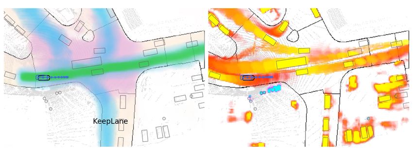
References                                                               [16] Noa Garnett, Rafi Cohen, Tomer Pe’er, Roee Lahav, and Dan
                                                                              Levi. 3d-lanenet: End-to-end 3d multiple lane detection. In
 [1] Zlatan Ajanovic, Bakir Lacevic, Barys Shyrokau, Michael                  Proceedings of the IEEE International Conference on Com-
     Stolz, and Martin Horn. Search-based optimal motion plan-                puter Vision, pages 2921–2930, 2019. 2
     ning for automated driving. In IROS, 2018. 1, 5
                                                                         [17] Andreas Geiger, Philip Lenz, and Raquel Urtasun. Are we
 [2] Min Bai, Gellert Mattyus, Namdar Homayounfar, Shenlong
                                                                              ready for autonomous driving? the kitti vision benchmark
     Wang, Shrinidhi Kowshika Lakshmikanth, and Raquel Ur-
                                                                              suite. In 2012 IEEE Conference on Computer Vision and
     tasun. Deep multi-sensor lane detection. In IROS, pages
                                                                              Pattern Recognition, pages 3354–3361. IEEE, 2012. 7
     3102–3109. IEEE, 2018. 2
                                                                         [18] Yuliang Guo, Guang Chen, Peitao Zhao, Weide Zhang, Jing-
 [3] Holger Banzhaf, Paul Sanzenbacher, Ulrich Baumann, and
                                                                              hao Miao, Jingao Wang, and Tae Eun Choe. Gen-lanenet:
     J. Marius Zöllner. Learning to predict ego-vehicle poses for
                                                                              A generalized and scalable approach for 3d lane detection.
     sampling-based nonholonomic motion planning. IEEE RA-L,
                                                                              arXiv, pages arXiv–2003, 2020. 2
     4(2):1053–1060, 2019. 3
                                                                         [19] Jeffrey Hawke, Richard Shen, Corina Gurau, Siddharth
 [4] Favyen Bastani, Songtao He, Sofiane Abbar, Mohammad
                                                                              Sharma, Daniele Reda, Nikolay Nikolov, Przemyslaw Mazur,
     Alizadeh, Hari Balakrishnan, Sanjay Chawla, Sam Madden,
                                                                              Sean Micklethwaite, Nicolas Griffiths, Amar Shah, et al. Ur-
     and David DeWitt. Roadtracer: Automatic extraction of road
                                                                              ban driving with conditional imitation learning. arXiv preprint
     networks from aerial images. In Proceedings of the IEEE
                                                                              arXiv:1912.00177, 2019. 2
     Conference on Computer Vision and Pattern Recognition,
     pages 4720–4728, 2018. 2                                            [20] Stefan Hoermann, Martin Bach, and Klaus Dietmayer. Dy-
 [5] Mariusz Bojarski, Davide Del Testa, Daniel Dworakowski,                  namic occupancy grid prediction for urban autonomous driv-
     Bernhard Firner, Beat Flepp, Prasoon Goyal, Lawrence D                   ing: A deep learning approach with fully automatic labeling.
     Jackel, Mathew Monfort, Urs Muller, Jiakai Zhang, et al.                 In 2018 IEEE International Conference on Robotics and Au-
     End to end learning for self-driving cars. arXiv preprint                tomation (ICRA), pages 2056–2063. IEEE, 2018. 2
     arXiv:1604.07316, 2016. 2, 3                                        [21] Namdar Homayounfar, Wei-Chiu Ma, Shrinidhi Kow-
 [6] Sergio Casas, Cole Gulino, Renjie Liao, and Raquel Ur-                   shika Lakshmikanth, and Raquel Urtasun. Hierarchical re-
     tasun. Spatially-aware graph neural networks for rela-                   current attention networks for structured online maps. In
     tional behavior forecasting from sensor data. arXiv preprint             Proceedings of the IEEE Conference on Computer Vision and
     arXiv:1910.08233, 2019. 2                                                Pattern Recognition, pages 3417–3426, 2018. 2
 [7] Sergio Casas, Cole Gulino, Simon Suo, Katie Luo, Renjie             [22] Namdar Homayounfar, Wei-Chiu Ma, Justin Liang, Xinyu
     Liao, and Raquel Urtasun. Implicit latent variable model                 Wu, Jack Fan, and Raquel Urtasun. Dagmapper: Learning
     for scene-consistent motion forecasting. arXiv preprint                  to map by discovering lane topology. In Proceedings of the
     arXiv:2007.12036, 2020. 2, 4                                             IEEE International Conference on Computer Vision, pages
 [8] Sergio Casas, Cole Gulino, Simon Suo, and Raquel Urtasun.                2911–2920, 2019. 2
     The importance of prior knowledge in precise multimodal             [23] Ajay Jain, Sergio Casas, Renjie Liao, Yuwen Xiong, Song
     prediction. arXiv preprint arXiv:2006.02636, 2020. 2                     Feng, Sean Segal, and Raquel Urtasun. Discrete residual
 [9] Sergio Casas, Wenjie Luo, and Raquel Urtasun. Intentnet:                 flow for probabilistic pedestrian behavior prediction. arXiv
     Learning to predict intention from raw sensor data. In CoRL,             preprint arXiv:1910.08041, 2019. 2
     2018. 2, 3, 11                                                      [24] Alex Kendall, Jeffrey Hawke, David Janz, Przemyslaw Mazur,
[10] Yuning Chai, Benjamin Sapp, Mayank Bansal, and Dragomir                  Daniele Reda, John-Mark Allen, Vinh-Dieu Lam, Alex Bew-
     Anguelov. Multipath: Multiple probabilistic anchor tra-                  ley, and Amar Shah. Learning to drive in a day. arXiv preprint
     jectory hypotheses for behavior prediction. arXiv preprint               arXiv:1807.00412, 2018. 3
     arXiv:1910.05449, 2019. 2, 4                                        [25] Alex H Lang, Sourabh Vora, Holger Caesar, Lubing Zhou,
[11] Felipe Codevilla, Matthias Miiller, Antonio López, Vladlen              Jiong Yang, and Oscar Beijbom. Pointpillars: Fast encoders
     Koltun, and Alexey Dosovitskiy. End-to-end driving via                   for object detection from point clouds. In Proceedings of the
     conditional imitation learning. In ICRA, 2018. 1, 2, 3, 7                IEEE Conference on Computer Vision and Pattern Recogni-
[12] Felipe Codevilla, Eder Santana, Antonio M López, and                    tion, pages 12697–12705, 2019. 2, 4
     Adrien Gaidon. Exploring the limitations of behavior cloning        [26] Lingyun Luke Li, Bin Yang, Ming Liang, Wenyuan Zeng,
     for autonomous driving. In Proceedings of the IEEE Inter-                Mengye Ren, Sean Segal, and Raquel Urtasun. End-to-end
     national Conference on Computer Vision, pages 9329–9338,                 contextual perception and prediction with interaction trans-
     2019. 3                                                                  former. arXiv preprint arXiv:2008.05927, 2020. 2
[13] Alberto Elfes. Using occupancy grids for mobile robot per-          [27] Junwei Liang, Lu Jiang, Kevin Murphy, Ting Yu, and Alexan-
     ception and navigation. Computer, 22(6):46–57, 1989. 2                   der Hauptmann. The garden of forking paths: Towards multi-
[14] Haoyang Fan, Zhongpu Xia, Changchun Liu, Yaqin Chen,                     future trajectory prediction. In Proceedings of the IEEE/CVF
     and Qi Kong. An auto-tuning framework for autonomous                     Conference on Computer Vision and Pattern Recognition,
     vehicles. arXiv preprint arXiv:1808.04913, 2018. 3                       pages 10508–10518, 2020. 2
[15] Davi Frossard, Simon Suo, Sergio Casas, James Tu, Rui Hu,           [28] Ming Liang, Bin Yang, Wenyuan Zeng, Yun Chen, Rui Hu,
     and Raquel Urtasun. Strobe: Streaming object detection from              Sergio Casas, and Raquel Urtasun. Pnpnet: End-to-end per-
     lidar packets. CoRL, 2020. 2                                             ception and prediction with tracking in the loop. In Proceed-

                                                                     9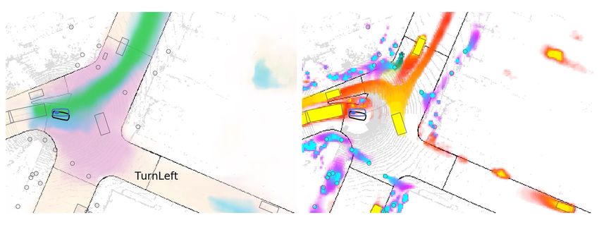
ings of the IEEE/CVF Conference on Computer Vision and               [43] Daniela Ridel, Nachiket Deo, Denis Wolf, and Mohan Trivedi.
       Pattern Recognition (CVPR), June 2020. 2                                  Scene compliant trajectory forecast with agent-centric spatio-
[29]   Rosanne Liu, Joel Lehman, Piero Molino, Felipe Petroski                   temporal grids. IEEE RA-L, 5(2):2816–2823, 2020. 2
       Such, Eric Frank, Alex Sergeev, and Jason Yosinski. An               [44] Stéphane Ross, Geoffrey Gordon, and Drew Bagnell. A re-
       intriguing failing of convolutional neural networks and the               duction of imitation learning and structured prediction to
       coordconv solution. In Advances in Neural Information Pro-                no-regret online learning. In Proceedings of the fourteenth in-
       cessing Systems, pages 9605–9616, 2018. 6, 11, 15                         ternational conference on artificial intelligence and statistics,
[30]   Wenjie Luo, Bin Yang, and Raquel Urtasun. Fast and furious:               pages 627–635, 2011. 2
       Real time end-to-end 3d detection, tracking and motion fore-         [45] Abbas Sadat, Sergio Casas, Mengye Ren, Xinyu Wu, Pranaab
       casting with a single convolutional net. In CVPR, 2018. 2, 3,             Dhawan, and Raquel Urtasun. Perceive, predict, and plan:
       4                                                                         Safe motion planning through interpretable semantic repre-
[31]   Huifang Ma, Yue Wang, Li Tang, Sarath Kodagoda, and                       sentations. In Proceedings of the European Conference on
       Rong Xiong. Towards navigation without precise localization:              Computer Vision (ECCV), 2020. 1, 2, 3, 4, 5, 7, 14
       Weakly supervised learning of goal-directed navigation cost          [46] Abbas Sadat, Mengye Ren, Andrei Pokrovsky, Yen-Chen Lin,
       map. CoRR, abs/1906.02468, 2019. 3                                        Ersin Yumer, and Raquel Urtasun. Jointly learnable behavior
                                                                                 and trajectory planning for self-driving vehicles. In IROS,
[32]   Sivabalan Manivasagam, Shenlong Wang, Kelvin Wong,
                                                                                 pages 3949–3956. IEEE, 2019. 1, 3, 5
       Wenyuan Zeng, Mikita Sazanovich, Shuhan Tan, Bin Yang,
       Wei-Chiu Ma, and Raquel Urtasun. Lidarsim: Realistic lidar           [47] Charlie Tang and Russ R Salakhutdinov. Multiple futures
       simulation by leveraging the real world. In Proceedings of                prediction. In Advances in Neural Information Processing
       the IEEE/CVF Conference on Computer Vision and Pattern                    Systems, pages 15398–15408, 2019. 2, 4
       Recognition, pages 11167–11176, 2020. 7                              [48] Sebastian Thrun. Learning occupancy grid maps with forward
[33]   Gellért Máttyus, Wenjie Luo, and Raquel Urtasun. Deep-                  sensor models. Autonomous robots, 15(2):111–127, 2003. 2
       roadmapper: Extracting road topology from aerial images. In          [49] Martin Treiber, Ansgar Hennecke, and Dirk Helbing. Con-
       Proceedings of the IEEE International Conference on Com-                  gested traffic states in empirical observations and microscopic
       puter Vision, pages 3438–3446, 2017. 2                                    simulations. Physical Review E, 62(2), Aug 2000. 8
[34]   Gregory P Meyer, Ankit Laddha, Eric Kee, Carlos Vallespi-            [50] Moritz Werling, Julius Ziegler, Sören Kammel, and Sebas-
       Gonzalez, and Carl K Wellington. Lasernet: An efficient prob-             tian Thrun. Optimal trajectory generation for dynamic street
       abilistic 3d object detector for autonomous driving. In Con-              scenarios in a frenet frame. In ICRA, 2010. 1, 5
       ference on Computer Vision and Pattern Recognition (CVPR),           [51] Pengxiang Wu, Siheng Chen, and Dimitris N Metaxas. Mo-
       pages 12677–12686. IEEE, 2019. 2, 4                                       tionnet: Joint perception and motion prediction for au-
                                                                                 tonomous driving based on bird’s eye view maps. In Pro-
[35]   Matthias Müller, Alexey Dosovitskiy, Bernard Ghanem, and
                                                                                 ceedings of the IEEE/CVF Conference on Computer Vision
       Vladen Koltun. Driving policy transfer via modularity and
                                                                                 and Pattern Recognition, pages 11385–11395, 2020. 2, 14
       abstraction. arXiv preprint arXiv:1804.09364, 2018. 3
                                                                            [52] Yuxin Wu and Kaiming He. Group normalization. In Proceed-
[36]   Tung Phan-Minh, Elena Corina Grigore, Freddy A Boulton,
                                                                                 ings of the European conference on computer vision (ECCV),
       Oscar Beijbom, and Eric M Wolff. Covernet: Multimodal
                                                                                 pages 3–19, 2018. 11
       behavior prediction using trajectory sets. arXiv preprint
                                                                            [53] Bin Yang, Wenjie Luo, and Raquel Urtasun. Pixor: Real-time
       arXiv:1911.10298, 2019. 2, 5
                                                                                 3d object detection from point clouds. In CVPR, 2018. 2, 3,
[37]   Jonah Philion and Sanja Fidler. Lift, splat, shoot: Encoding              4, 11
       images from arbitrary camera rigs by implicitly unproject-
                                                                            [54] Fisher Yu and Vladlen Koltun.              Multi-scale context
       ing to 3d. In Proceedings of the European Conference on
                                                                                 aggregation by dilated convolutions.            arXiv preprint
       Computer Vision, 2020. 2, 5, 7, 8
                                                                                 arXiv:1511.07122, 2015. 11
[38]   Philip Polack, Florent Altché, Brigitte d’Andréa Novel, and        [55] Wenyuan Zeng, Wenjie Luo, Simon Suo, Abbas Sadat, Bin
       Arnaud de La Fortelle. The kinematic bicycle model: A                     Yang, Sergio Casas, and Raquel Urtasun. End-to-end inter-
       consistent model for planning feasible trajectories for au-               pretable neural motion planner. In CVPR, 2019. 3, 5, 7,
       tonomous vehicles? In 2017 IEEE Intelligent Vehicles Sym-                 8
       posium (IV), pages 812–818. IEEE, 2017. 5
                                                                            [56] Tianyang Zhao, Yifei Xu, Mathew Monfort, Wongun Choi,
[39]   Dean A Pomerleau. Alvinn: An autonomous land vehicle in                   Chris Baker, Yibiao Zhao, Yizhou Wang, and Ying Nian Wu.
       a neural network. In NIPS, 1989. 2                                        Multi-agent tensor fusion for contextual trajectory prediction.
[40]   Nathan D Ratliff, J Andrew Bagnell, and Martin A Zinkevich.               In Proceedings of the IEEE Conference on Computer Vision
       Maximum margin planning. In ICML, 2006. 7, 14                             and Pattern Recognition, pages 12126–12134, 2019. 2
[41]   Nicholas Rhinehart, Kris M Kitani, and Paul Vernaza. R2p2:           [57] Yin Zhou, Pei Sun, Yu Zhang, Dragomir Anguelov, Jiyang
       A reparameterized pushforward policy for diverse, precise                 Gao, Tom Ouyang, James Guo, Jiquan Ngiam, and Vijay
       generative path forecasting. In ECCV, 2018. 2, 4                          Vasudevan. End-to-end multi-view fusion for 3d object detec-
[42]   Nicholas Rhinehart, Rowan McAllister, and Sergey Levine.                  tion in lidar point clouds. arXiv preprint arXiv:1910.06528,
       Deep imitative models for flexible inference, planning, and               2019. 2, 4
       control. arXiv preprint arXiv:1810.06544, 2018. 4

                                                                       10
Appendix a 1-layer CNN outputs the current occupancy map, a 2-layer
CNN the motion mode scores for all time steps, and another
In this appendix we first explain our implementation de- 2-layer CNN the motion vectors for all modes and future
tails in depth, then showcase additional experiments to pro- time steps. We employ dilation [54] to increase the receptive
vide more insights from our model, and finally provide addi- field while keeping the number of parameters low in order
tional qualitative results. to be able to predict motion for voxels that are far away
from the original position of actors for the long temporal
horizons. To infer the future occupancy, we simply warp the
A. Implementation details initial occupancy with the temporal motion field as explained
A.1. Architecture in the main manuscript’s Fig. 3.4., and further detailed in
Section A.2. In practice, we found that K = 3 modes was
Backbone network: Fig. 6 shows an architecture diagram expressive enough for the multi-modality of the temporal
of the backbone network. We combine ideas from [9, 53] motion field. In all our experiments, T = 11 since we predict
to build a multi-resolution backbone network that extracts the future 5 seconds at 0.5-second intervals.
geometric and semantic information from the past LiDAR
sweeps and is able to aggregate them to reason about motion.
Our backbone is composed of 4 convolutional blocks, and Routing architecture: In order to drive towards a goal,
a convolutional header. The number of output features and we would like to follow the driving commands. To do so,
kernel size is indicated in Fig. 6. All convolutional layers we predict a route spatial map, where each cell represents
use Group Normalization [52] with 32 groups, and ReLU the probability that driving to it from the current location
non-linearity. The scene context features after each residual is aligned with the driving command. The architecture for
block are C1x , C2x , C4x , C8x , where the subscript indicates the network that predicts such spatial map is detailed in
the downsampling factor from the input in BEV. The features 9. The high-level action in the command acts as a switch
from the different blocks are then concatenated at 4x down- between 3 instantiations of the same network architecture
sampling by max-pooling higher resolution ones C1x , C2x (i.e., one for turning right, one for turning left, one for going
and interpolating C8x . Finally, a residual block of 4 con- straight). The longitudinal distance to action is repeated spa-
volutional layers with no downsampling outputs the scene tially with the same resolution as the online map. Then, both
context C. Since the LiDAR input is voxelized at 0.2 meters are concatenated to form the input to a CNN that leverages
per pixel, C has a resolution of 0.8 meters per pixel. Coordinate Convolutions (CoordConv) [29] in order to be
able to reason about the distance to a particular grid cell
from the SDV.
Mapping architecture: In order to drive safely (e.g., nar-
row streets) we need a high resolution representation of our A.2. Dynamic occupancy
maps, and at the same time a big receptive field to help
reduce uncertainty (e.g., around occlusions). To achieve Here we provide a more detailed explanation of how our
this efficiently, we employ a multi-resolution architecture dynamic occupancy flow works than in the main manuscript.
as shown in Fig. 7. It takes as input multiple feature maps We first define a flow event from spatio-temporal grid cell
C1x , C2x , C from the backbone network (see Fig. 6), and out- (t, i1 ) to (t + 1, i2 ) as the intersection of the event that the
puts the 6 channels of the online map at the original input original grid cell is occupied, and that the motion field moves
resolution of 0.2 m/pixel. As a reminder, the six channels this occupancy from (t, i1 ) to (t + 1, i2 ). Since we consider
are: 1 for drivable area score, 1 for intersection score, 2 K motion modes, the final flow event considers the union of
for truncated unsigned distance reachable lane (mean and those, effectively marginalizing over modes:
variance of Gaussian distribution), 2 for the angle to closest
reachable lane segment (location and concentration of Von F(t,i1 )→(t+1,i2 ) = ∪k {Oit1 ∩ Kit1 = k ∩ Vit,k
1
= i2 }
Mises distribution).
Given this flow event definition and the assumptions in our
probabilistic model, we can obtain its probability:
Perception and Prediction architecture: The different X
c c c c
dynamic classes (i.e. vehicles, pedestrians and bicyclists) p(F(t,i 1 )→(t+1,i2 )
)= p(Ot,i 1
)p(Kt,i 1
= k)p(Vt,i 1 ,k
= i2 )
are processed by different networks since they have very k
different geometry as well as motion. For each class, a
2-layer CNN processes C and upsamples it to 0.4 m/pixel. We can now calculate the future occupancy iteratively,
This is the same resolution as C2x , which gets processed starting from the occupancy predictions at t = 0. Specif-
by another 2-layer CNN. Then the two feature maps get ically, to get the occupancy that flows into cell i at time
concatenated to form the dynamic context. From this context, t + 1 from all cells j at time t, we can simply compute the
11Figure 6: Backbone Network. The output features within one CNN block are fixed. All kernel strides and dilation are 1.
128, 3x3, 2 128, 3x3, 1 128, 3x3, 1 6, 3x3, 1
Conv2d + GroupNorm + ReLU Conv2d Interpolate Concat Output features, kernel size, dilation
Figure 7: Mapping Network. The output features within one CNN block are fixed. All kernel strides are 1.
probability that no occupancy flow event occurs, and take its of trajectories are influenced by the initial state, resulting in
complement kinematically-plausible trajectory sampling.
c
p(Ot+1,i ) = p ∪j F(t,j)→(t+1,i) : ∀k, l
0 A.3.2 Trajectory Scoring
= 1 − p ∩j F(t,j)→(t+1,i) : ∀k, l
Y
c
In the following, we provide more details about the cost
=1− 1 − p(F(t,j)→(t+1,i) ) function of the planner.
j
0
where F(t,j)→(t+1,i) denotes the complement of Reachable-lanes direction In addition to stay close to the
F(t,j)→(t+1,i) . lane centerlines, we promote trajectories that stay aligned
with the direction of the lane. Towards this goal, we use the
A.3. Planning average difference of the trajectory point heading and the
In this section we provide more details about trajectory angles in Mθ indexed at all BEV grid-cells that have overlap
retrieval and the coring functions. with SDV polygon.
fd (x, M) = E |Mθi − xθ |
A.3.1 Trajectory Retreival i∈m(x)
We use ∼ 150 hours of manual driving data to create the
where m(x) represents the spatial indices of BEV grid-cells
dataset of expert trajectories. To group the trajectories into
of the map-layer prediction that overlaps with SDV polygon
different bins, we use the initial velocity v, curvature κ, and
with state x.
acceleration a, with respective bin sizes of 2.0 m 1
s , 0.02 m ,
m
and 1.0 s2 . The trajectories in each bins are clustered into
3, 000 sets and the closest trajectory to each cluster prototype Lane uncertainty In order to promote cautious behavior
is kept. This creates a set fo diverse trajectories conditioned when there is high uncertainty in MD and Mθ , we use a
on the current state of SDV. Figure 10 shows example sets of cost function that is the product of the SDV velocity and the
trajectories retrieved base on the indicated initial state (initial standard deviation of the probability distributions of cells
acceleration is 0.0 in all the cases). We can see how the set overlapping with SDV in MD and Mθ . This promotes slow
12You can also read