Multi-Objective Optimization of Cutting Parameters in Turning AISI 304 Austenitic Stainless Steel - MDPI
←
→
Page content transcription
If your browser does not render page correctly, please read the page content below
metals
Article
Multi-Objective Optimization of Cutting Parameters
in Turning AISI 304 Austenitic Stainless Steel
Yu Su, Guoyong Zhao *, Yugang Zhao, Jianbing Meng             and Chunxiao Li
 School of Mechanical Engineering, Shandong University of Technology, Zibo 255000, China;
 18753391805@163.com (Y.S.); zhaoyg9289@126.com (Y.Z.); jianbingmeng@126.com (J.M.);
 19862576051@163.com (C.L.)
 * Correspondence: zgy709@sdut.edu.cn; Tel.: +86-0533-278-7910

 Received: 17 January 2020; Accepted: 1 February 2020; Published: 3 February 2020

 Abstract: Energy conservation and emission reduction is an essential consideration in sustainable
 manufacturing. However, the traditional optimization of cutting parameters mostly focuses on
 machining cost, surface quality, and cutting force, ignoring the influence of cutting parameters on
 energy consumption in cutting process. This paper presents a multi-objective optimization method
 of cutting parameters based on grey relational analysis and response surface methodology (RSM),
 which is applied to turn AISI 304 austenitic stainless steel in order to improve cutting quality and
 production rate while reducing energy consumption. Firstly, Taguchi method was used to design the
 turning experiments. Secondly, the multi-objective optimization problem was converted into a simple
 objective optimization problem through grey relational analysis. Finally, the regression model based
 on RSM for grey relational grade was developed and the optimal combination of turning parameters
 (ap = 2.2 mm, f = 0.15 mm/rev, and v = 90 m/s) was determined. Compared with the initial turning
 parameters, surface roughness (Ra) decreases 66.90%, material removal rate (MRR) increases 8.82%,
 and specific energy consumption (SEC) simultaneously decreases 81.46%. As such, the proposed
 optimization method realizes the trade-offs between cutting quality, production rate and energy
 consumption, and may provide useful guides on turning parameters formulation.

 Keywords: AISI 304 austenitic stainless steel; multi-objective optimization; cutting parameters;
 specific energy consumption; grey relational analysis; response surface methodology (RSM)

1. Introduction
     Cutting process is the main means of mechanical manufacturing, which plays an important
role in the manufacturing industry. It was found that the formulation of cutting parameters has
significant influence on cutting quality, production rate, and energy consumption [1–3]. In general,
most of the cutting parameters are determined according to engineering experience and specialized
handbooks, which cannot obtain the optimal machining effect. Consequently, the optimization of
cutting parameters for different objectives has always been a hot issue in manufacturing enterprises
and academia.
     The surface integrity, machining efficiency, and cutting force are usually taken as objectives in
most of the traditional optimization of cutting parameters. For example, Kumar [4] adopted surface
roughness and material removal rate (MRR) as objectives to optimize the cutting parameters in turning
C360 copper alloy. Zhou et al. [5] obtained the Pareto optimal solution with the maximum MRR and
the minimum surface roughness in turning AISI 304 based on the genetic algorithm gradient boosting
regression tree (GA-GBRT) model they established. Their experimental results demonstrated that MRR
can be improved by increasing cutting depth and cutting speed in a small range of surface roughness
variations. In addition, the grey relational analysis is often used as a powerful tool when dealing with

Metals 2020, 10, 217; doi:10.3390/met10020217                                   www.mdpi.com/journal/metals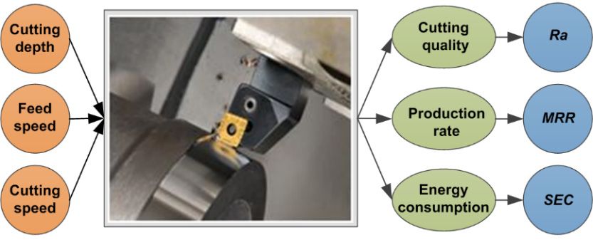
Metals 2020, 10, 217                                                                                 2 of 11

multi-objective optimization of cutting parameters. Using grey relational analysis, Li and Wang [6]
optimized the grinding parameters, which effectively reduces the workpiece surface roughness and
flatness. Kuram and Ozcelik [7] measured MRR, cutting force, and surface roughness in micro-milling
Al 7075 and used grey relational analysis to determine the optimal combination of milling parameters
with these three machining characteristics as objectives. Significant work has been carried out based
on machining science and cost consideration. However, the influence of cutting parameters on energy
consumption in cutting process is not considered in the aforementioned research.
      The rapid development of the manufacturing industry has brought great convenience to
human society, while exacerbating the problem of resource shortage and environmental pollution as
well [2]. As the basic unit in machining systems, machine tool has large quantity with high energy
consumption [8]. Vijayaraghavan et al. [9] suggested that reducing the energy consumption of machine
tool can dramatically improve the environmental performance of the manufacturing industry. Thus,
many scholars have studied energy consumption characteristics of machine tool in order to improve
the energy efficiency of machine tool. Based on the investigation of the relationship between energy
consumption of machine tool and MRR, Kara and Li [10] proposed an energy consumption prediction
model suitable for turning and milling processes. On this basis, Li et al. [11] improved the energy
consumption prediction model of milling processes with taking the spindle speed into consideration.
Moreover, Zhang et al. [12] developed the specific energy consumption (SEC) model based on cutting
parameters and analyzed the influence of cutting parameters on SEC. These research projects show that
the energy consumption of machine tool can be reduced by selecting reasonable cutting parameters,
laying the foundation for energy efficiency optimization of machine tool.
      Recently, the optimization of cutting parameters aiming at energy saving and emission reduction
has become a research hotspot in sustainable manufacturing. For reducing the energy consumption
of machine tool, Camposeco-Negrete [13] optimized the cutting parameters in turning of AISI 6061
T6 aluminum by using Taguchi method and ANOVA. His research also pointed out that higher feed
speed provides minimum energy consumption but will lead to higher surface roughness. It is worth
noticing that the optimal cutting parameters for one machining characteristic may worsen other
machining characteristics. Hence, the multi-objective optimization of cutting parameters based on
both technique requirements and energy-saving consideration is more reasonable in actual machining.
Zhao et al. [14] optimized the milling parameters through grey relational analysis, which can reduce
energy consumption and improve surface quality simultaneously. In order to minimize the cutting
time and energy consumption per unit of removed material, Zhou et al. [15] proposed a multi-objective
optimization model and obtained the optimal cutting parameters by genetic algorithm (GA). Similarly,
Li et al. [16] established the RSM models of energy efficiency and cutting time, and optimized milling
parameters through particle swarm optimization algorithm (PSOA). Yan and Li [17] presented an
approach for optimization of milling parameters with multiple responses such as cutting energy
consumption, surface roughness, and MRR, which integrated the weighted grey relational analysis
and RSM. Furthermore, Li et al. [18] explored the influence of cutting parameters on tool wear and
surface topography in turning AISI 304, and optimized the cutting parameters with the goal of the
maximum MRR and the minimum specific cutting energy.
      Based on the above literature, it is noted that the optimization of cutting parameters has
changed from single objective optimization to multi-objective optimization considering both technique
requirements and environmental performance. Although recent work has made valuable contributions
towards energy conservation and emission reduction, the optimization of cutting parameters for
sustainable manufacturing requires more comprehensive study, especially for some difficult-to-machine
materials. Therefore, the objectives of this paper are to: (1) Investigate the multi-objective optimization
framework of turning parameters for sustainable manufacturing; (2) propose the multi-objective
optimization method based on grey relational analysis and RSM; (3) verify the optimization method
with wet turning experiments of AISI 304 austenitic stainless steel.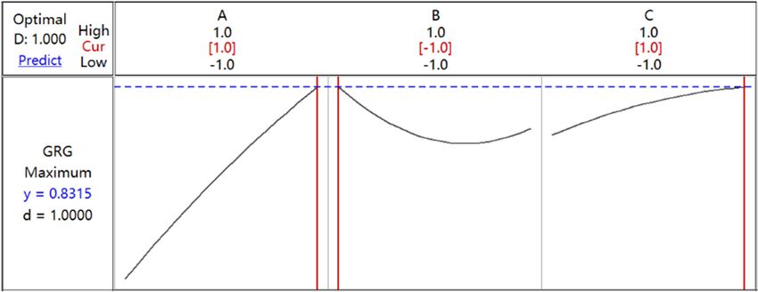
Metals 2020, 10, 217 3 of 11
Metals 2020, 10, 217 3 of 12
2. Multi-Objective Optimization Framework of Turning Parameters
2. Multi-Objective Optimization Framework of Turning Parameters
Lathes account for about 20–35% of the total number of cutting machine tool. They are mainly
used Lathes accountvarious
for machining for about 20–35%
rotating of the such
surfaces, total asnumber
internal of cylindrical
cutting machine tool.
surfaces, They are
external mainly
cylindrical
used for machining various rotating surfaces, such as internal cylindrical
surfaces, and conical surfaces. The traditional turning process improves production rate as much as surfaces, external
cylindrical
possible onsurfaces, and of
the premise conical surfaces.the
guaranteeing Thecutting
traditional turning
quality. processthe
However, improves production rate
energy consumption of
as much tool
machine as possible on the effects
and the adverse premiseon oftheguaranteeing
environment are the ignored.
cutting quality. However, the energy
consumption of machine
In a specific machiningtoolsystem,
and thetheadverse
selection effects on the parameters
of cutting environment are ignored.
becomes the basis of process
In a specificFor
optimization. machining system,
the turning the selection
process orientedoftocutting parameters
sustainable becomes thethe
manufacturing, basis of process
optimization
optimization.
objectives Forbethe
should turning toprocess
expanded cutting oriented to sustainable
quality, production manufacturing,
rate, and the optimization
energy consumption. Surface
objectives should be expanded to cutting quality, production rate, and energy
roughness, MRR, and SEC are featured as evaluation criteria of machining characteristics. Therefore,consumption. Surface
roughness,
the MRR, and
multi-objective SEC are featured
optimization frameworkas evaluation
of turningcriteria of machining
parameters characteristics.
can be outlined in FigureTherefore,
1 and the
the multi-objective optimization framework
optimization problem can be described as Equation (1). of turning parameters can be outlined in Figure 1 and
the optimization problem can be described as Equation (1).
minRa (ap(a, f,f,v)
, v)
min Ra p a≤
a ap ≤≤aapp ≤ apmax
pmin
p
min
max
maxMRR ( a , f , v ) f f ≤≤ fmax
f ≤ f max (1)
max MRRp(ap ,f,v) f ≤min
(1)
min
minSEC
(ap , pf,f,v)
min SEC(a , v)
vmin ≤ vmin
v ≤≤vmaxv ≤ vmax
where Ra
where Ra is
is surface roughness, MRR
surface roughness, MRR is is material
material removal rate, SEC
removal rate, SEC is
is specific
specific energy
energy consumption
consumption of
of
machine tool, a is cutting depth, f is feed speed, and v is cutting speed.
machine tool, app is cutting depth, f is feed speed, and v is cutting speed.
Figure
Figure 1. Multi-objective optimization
1. Multi-objective optimization framework
framework of
of turning
turning parameters.
parameters.
2.1. Cutting Quality
2.1. Cutting Quality
The surface quality usually has a great influence on mechanical performance of parts [19]. It has
The surface quality usually has a great influence on mechanical performance of parts [19]. It has
been proved that the scrapping of many mechanical products is caused by the surface defects of
been proved that the scrapping of many mechanical products is caused by the surface defects of parts.
parts. Surface roughness is therefore considered as a vital technical requirement in cutting process.
Surface roughness is therefore considered as a vital technical requirement in cutting process.
Moreover, it was found that surface roughness is closely related to cutting conditions, especially cutting
Moreover, it was found that surface roughness is closely related to cutting conditions, especially
parameters [20].
cutting parameters [20].
2.2. Production Rate
2.2. Production Rate
MRR, as one of the criteria for evaluating production rate, is widely used for cutting process
MRR, as one
optimization. of the
While the criteria for evaluating
traditional selection ofproduction rate, is widely
cutting parameters used for cutting
is conservative, whichprocess
is not
optimization. While the traditional selection of cutting parameters is conservative, which is not
conducive to the realization of efficient machining. The value of MRR when turning external cylindrical
conducive
surface can to the realization
be calculated usingof efficient(2).machining. The value of MRR when turning external
Equation
cylindrical surface can be calculated using Equation (2).
2 2
π[( dd) 2 − ( dd− ap ) 2]n f
MRR = π[(22) − (22 − a ) ]nf (2)
MRR = 60
60
where d is workpiece diameter in mm, n
where d is workpiece diameter in mm, n is spindle speedininrev/min,
is spindle speed rev/min,f is
f isfeed speed
feed inin
speed mm/rev, and
mm/rev, ap
and
is cutting depth in mm.
ap is cutting depth in mm.
2.3. Energy Consumption
In general, the cutting stage is the most energy-consuming work process of machine tool. In this
stage, the energy consuming components include machine control unit (MCU), spindle motor, feed-Metals 2020, 10, 217 4 of 11
2.3. Energy Consumption
In general, the cutting stage is the most energy-consuming work process of machine tool. In this
stage, the energy consuming components include machine control unit (MCU), spindle motor, feed-axis
motors, cooling pump motor, and lighting device. The energy consumption can be obtained by
monitoring the power consumption of machine tool [21].
SEC expresses the required energy consumption when cutting unit volume material and can
be computed by Equation (3). Moreover, the advantage of SEC is that as long as the specific
energy consumption is achieved, the machine tool energy consumption in machining can be
predicted accurately.
E P·t P
SEC = = = (3)
Q MRR·t MRR
where E is machine tool energy consumption in J, Q is material removal volume in mm3 , P is total
power of machine tool in cutting stage in W, MRR is material removal rate in mm3 /s, and t is cutting
time in s.
3. Optimization Example
3.1. Experimental Details
3.1.1. Workpiece Material and Cutting Tool
AISI 304 austenitic stainless steel is used widely in machinery, aerospace, and medical
device industry because of its good overall performance. However, it also belongs to one of the
difficult-to-machine materials due to its high toughness, serious work hardening, and bad thermal
conductivity. AISI 304 was chosen as workpiece material, and its chemical composition and physical
properties are shown in Tables 1 and 2. In addition, the workpiece diameter is 55 mm and cutting
length is 120 mm. The experiments were carried out with hard alloy external turning inserts CNMG
120408–PG SC2035.
Table 1. Chemical composition of AISI 304 austenitic stainless steel.
Composition C Mn Si P S Ni Cr Mo Cu Fe
wt% 0.065 1.78 0.3 0.027 0.02 8.1 18.2 0.13 0.14 71.2
Table 2. Physical properties of AISI 304 austenitic stainless steel.
Specific Heat Capacity Elastic Modulus Coefficient of Thermal Expansion Thermal Conductivity Density
(J·kg−1 ·K−1 ) (GPa) (10−6 ·K−1 ) (W·m−1 ·K−1 ) (g/cm3 )
500 194 17.3 16.3 7.93
3.1.2. Experimental Equipment
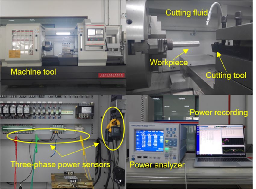
Wet turning AISI 304 round bars and power measurement were performed and are shown in
Figure 2. The computer numerical control (CNC) lathe is Yishui CKJ6163 (Yishui Inc., Shandong, China),
with a maximum spindle speed of 1000 rev/min, a maximum spindle power of 11 kW, and a cooling
pump power of 0.125 kW. The power analyzer WT500 (Yokogawa, Tokyo, Japan) and sensors were
adopted to measure power consumption from the lathe input lines. Three-phase power signals were
connected to WT500 and recorded with WTViewerEfree software. In addition, the surface roughness
tester RTP120 (Shjingmi Inc., Shanghai, China) was employed to measure the workpiece machined
surface roughness.Metals 2020, 10, 217 5 of 11
Metals 2020, 10, 217 5 of 12
Figure
Figure 2. Experimentalprocessing
2. Experimental processing and
and measuring
measuringequipment.
equipment.
3.1.3. 3.1.3.
Design Design of Experiments
of Experiments
The variances
The variances of cutting
of cutting depth
depth ap ,afeed
p, feed speedf, f,and
speed andcutting
cutting speed
speed vv were
werecustomized
customizedaccording
according to
to the capacity of the lathe and the cutting inserts. Table 3 shows the cutting parameters
the capacity of the lathe and the cutting inserts. Table 3 shows the cutting parameters and their and their
levels.
levels. Taguchi method was used to design the3 L25 (53) orthogonal experiments with three factors and
Taguchi method was used to design the L25 (5 ) orthogonal experiments with three factors and five
five levels, as shown in Table 4. The initial cutting parameter used the recommended value, cutting
levels, as shown in Table 4. The initial cutting parameter used the recommended value, cutting depth
depth of 1.2 mm, feed speed of 0.25 mm/rev, and cutting speed of 90 m/min.
of 1.2 mm, feed speed of 0.25 mm/rev, and cutting speed of 90 m/min.
Table 3. Cutting parameters and their levels.
Table 3. Cutting parameters and their levels.
Parameters Range Level 1 Level 2 Level 3 Level 4 Level 5
Parametersap (mm)
Range 0.2–2.2 Level 1 0.2 Level 0.7
2 Level
1.2 3 Level 4
1.7 2.2 Level 5
ap (mm)f (mm/rev)
0.2–2.2 0.15–0.35
0.2 0.15 0.7 0.20 0.25
1.2 0.301.7 0.35 2.2
f (mm/rev) 0.15–0.35
v (m/min) 50–900.15 50 0.20
60 0.25
70 800.30 90 0.35
v (m/min) 50–90 50 60 70 80 90
Before each set of experiments, the spindle speed was calculated according to Equation (4) for
Table 4. Experiment design using L25 (53 ) orthogonal array and their measurement results.
CNC programming.
ap f v d 1000v n Ra MRR SEC
No. n= (4)
(mm) (mm/rev) (m/min) (mm) πd (r/min) (µm) (mm3 /s) (J/mm3 )
where v is1 cutting speed
0.2 0.15
in m/min, 50
d is workpiece 47.40
diameter336 1.0325
in mm, and 24.9116 speed
n is spindle 73.8180
in rev/min.
2 0.2 0.20 60 46.97 407 1.5835 39.8676 56.2968
After3 each set0.2of experiments,
0.25 the
70 workpiece
46.55 surface
479 roughness
2.3270 was measured
58.1238 from
46.4650 three
different locations,
4 and the average
0.2 0.30 value
80 was taken
46.13 as the621
surface roughness
3.0725 Ra in each
89.6062 experiment.
39.1952
The MRR 5and SEC 0.2 under each 0.35 90
set of cutting 45.71
parameters 627
were 3.9995
obtained 104.5854
according 34.9219
to Equation (2) and
6 0.7 0.15 60 45.29 422 0.9995 103.4517 25.0040
(3), respectively.
7 Twenty-five
0.7 sets
0.20 of experimental
70 results
43.87 are
508 summarized
1.6190 in Table
160.7579 4. 19.7991
8
Because 0.7 of workpiece
the size 0.25 was80 small and42.44 600
turning experiments 2.3195 229.4776
were performed 16.4892
using cutting
9 0.7 0.30 90 41.03 699 3.0820 309.9726 14.3977
fluid, the 10
tool wear0.7
was not serious.
0.35
In addition,
50
all experiments
39.60 402
used new
3.8170
cutting inserts
200.6044
and the tool
13.6178
flank wear 11 was less
1.2than 0.10 mm.
0.15 Therefore,
70 the influence
38.17 584 of tool wear
0.8830 was not
203.4855 considered
18.3305 in the
paper. 12 1.2 0.20 80 35.74 713 1.6265 309.4723 14.9285
13 1.2 0.25 90 33.32 860 2.4110 433.9042 13.2391
14 1.2 0.30 50 30.93 515 3.1150 288.6046 12.3712
15 1.2 0.35 60 46.98 407 3.8100 409.7492 1.4578
16 1.7 0.15 80 44.56 572 0.7810 327.3309 1.9894
17 1.7 0.20 90 41.14 697 1.4180 489.3811 1.5024
18 1.7 0.25 50 37.67 423 2.1520 338.5855 2.3185
19 1.7 0.30 60 34.28 557 3.0020 484.5907 1.4280
20 1.7 0.35 70 30.90 721 3.8335 655.8941 1.1752
21 2.2 0.15 90 46.85 612 0.7980 472.1559 2.4545
22 2.2 0.20 50 42.40 376 1.4105 348.2292 3.1293
23 2.2 0.25 60 37.03 516 1.7555 517.5645 2.1792
24 2.2 0.30 70 32.58 684 2.8110 718.1025 1.4547
25 2.2 0.35 80 43.53 585 3.6870 974.7890 1.1535Metals 2020, 10, 217 6 of 11
Before each set of experiments, the spindle speed was calculated according to Equation (4) for
CNC programming.
1000v
n= (4)
πd
where v is cutting speed in m/min, d is workpiece diameter in mm, and n is spindle speed in rev/min.
After each set of experiments, the workpiece surface roughness was measured from three different
locations, and the average value was taken as the surface roughness Ra in each experiment. The MRR
and SEC under each set of cutting parameters were obtained according to Equation (2) and (3),
respectively. Twenty-five sets of experimental results are summarized in Table 4.
Because the size of workpiece was small and turning experiments were performed using cutting
fluid, the tool wear was not serious. In addition, all experiments used new cutting inserts and the
tool flank wear was less than 0.10 mm. Therefore, the influence of tool wear was not considered in
the paper.
3.2. Grey Relational Analysis
The advantage of grey relational analysis is that it can transform the complex multi-objective
optimization problem into a single objective optimization problem through the calculation of grey
relational grade (GRG). The calculation of GRG includes the following three steps [22].
Firstly, preprocess the experimental results of Ra, MRR, and SEC to avoid the effect of adopting
different units. If the original data sequence is ‘the-smaller-the-better’, then this original data sequence
is preprocessed using Equation (5); if the original data sequence is ‘the-larger-the-better’, then this
original data sequence is preprocessed using Equation (6).
◦ ◦
maxxi (k) − xi (k)
x∗i (k) = ◦ ◦ (5)
maxxi (k) − minxi (k)
◦ ◦
xi (k) − minxi (k)
x∗i (k) = ◦ ◦ (6)
maxxi (k) − minxi (k)
i = 1, 2, . . . , m; k = 1, 2, . . . , z (7)
◦
where m is the number of experiments, z is the number of data sequences, xi (k) is the original data
◦ ◦
sequence, maxxi (k) is the maximum value in the original data sequence, minxi (k) is the minimum
value in the original data sequence, and x∗i (k) is the contrast sequence. In this optimization example, the
smaller Ra, the larger MRR, and the smaller SEC are desired. Therefore, the data sequences Ra, MRR,
and SEC were preprocessed by Equation (5), Equation (6), and Equation (5), respectively. The results of
data preprocessing are shown in Table 5.
Secondly, calculate the grey relational coefficient (GRC) based on the results of data preprocessing.
∆min + ϕ∆max
ξi ( k ) = (8)
∆oi (k)+ϕ∆max
∆oi (k) = Xo (k)−x∗i (k) (9)
∆min =min min Xo (k)−x∗j (k) (10)
∀j∈i ∀k
∆max =max max Xo (k)−x∗j (k) (11)
∀ j∈i ∀k
where ξi (k) is GRC, Xo (k) is the reference sequence and Xo (k) = 1, ∆oi (k) is the deviation value
between Xo (k) and x∗i (k), and ϕ is the distinguishing coefficient and ϕ = 0.5 normally.Metals 2020, 10, 217 7 of 11
Table 5. The results of data preprocessing.
Contrast Sequence Ra MRR SEC
1 0.9219 0.0000 0.0000
2 0.7507 0.0157 0.2411
3 0.5197 0.0350 0.3764
4 0.2880 0.0681 0.4765
5 0.0000 0.0839 0.5353
6 0.9321 0.0827 0.6718
7 0.7396 0.1430 0.7434
8 0.5220 0.2154 0.7890
9 0.2851 0.3001 0.8177
10 0.0567 0.1850 0.8285
11 0.9683 0.1880 0.7636
12 0.7373 0.2996 0.8104
13 0.4936 0.4306 0.8337
14 0.2748 0.2776 0.8456
15 0.0589 0.4051 0.9958
16 1.0000 0.3184 0.9885
17 0.8021 0.4890 0.9952
18 0.5740 0.3302 0.9840
19 0.3099 0.4839 0.9962
20 0.0516 0.6643 0.9997
21 0.9947 0.4708 0.9821
22 0.8044 0.3404 0.9728
23 0.6972 0.5186 0.9859
24 0.3693 0.7298 0.9959
25 0.0971 1.0000 1.0000
Finally, calculate the grey relation grade (GRG) according to the values of GRC and weights.
z
X
γi = wk ξi (k) (12)
k=1
z
X
wk = 1 (13)
k=1
where γi is GRG and wk is weight. The weight of the output can be determined by the expert system
according to actual production demand. In this optimization example, the weights of the three
optimization objectives are the same, namely w1 :w2 :w3 = 1:1:1.
The gray correlation coefficients (GRCMRR , GRCRa , and GRCSEC ) and GRG of each set of
experiments can be obtained by Equations (8)–(13). The results of grey relational analysis and sorting
of GRG are shown in Table 6.
3.3. Process Modelling and ANOVA
The original relationship between cutting parameters and three optimization objectives has been
transformed into a new relationship between cutting parameters and GRG through grey relational
analysis. In order to find the optimal cutting parameters, the regression model of GRG based on
cutting parameters needs to be established first. The RSM was applied to fit the regression model, and
Equation (14) represents the general form of the second-order RSM model.
k
X XX k
X
y = β0 + βi xi + βij xi x j + βii x2i + ε (14)
i=1 iMetals 2020, 10, 217 8 of 11
where x are independent variables, namely cutting parameters, k is the number of independent
variables, β is a coefficient of each term, and ε is a residual error.
Table 6. Results of grey relational analysis.
Contrast Sequence GRCMRR GRCRa GRCSEC GRG Sort
1 0.3333 0.8648 0.3333 0.5105 20
2 0.3369 0.6673 0.3972 0.4671 22
3 0.3413 0.5100 0.4450 0.4321 23
4 0.3492 0.4125 0.4885 0.4167 24
5 0.3531 0.3333 0.5183 0.4016 25
6 0.3528 0.8805 0.6037 0.6123 12
7 0.3685 0.6576 0.6609 0.5623 16
8 0.3892 0.5112 0.7032 0.5345 17
9 0.4167 0.4115 0.7329 0.5204 19
10 0.3802 0.3464 0.7446 0.4904 21
11 0.3811 0.9404 0.6790 0.6668 8
12 0.4165 0.6556 0.7251 0.5991 13
13 0.4675 0.4968 0.7504 0.5716 15
14 0.4090 0.4081 0.7641 0.5271 18
15 0.4567 0.3470 0.9917 0.5984 14
16 0.4231 1.0000 0.9775 0.8002 2
17 0.4945 0.7164 0.9905 0.7338 4
18 0.4274 0.5400 0.9689 0.6454 10
19 0.4921 0.4201 0.9925 0.6349 11
20 0.5983 0.3452 0.9994 0.6476 9
21 0.4858 0.9895 0.9654 0.8136 1
22 0.4312 0.7188 0.9484 0.6995 6
23 0.5095 0.6228 0.9725 0.7016 5
24 0.6492 0.4422 0.9918 0.6944 7
25 1.0000 0.3564 1.0000 0.7855 3
The cutting depth, feed speed, and cutting speed were coded using Equations (15)–(17), respectively.
The values of cutting parameters were normalized to the range of −1 to 1, which could cause the
controlled factors to affect the responses more evenly [23]. The software Minitab17 was applied to fit
the experimental data, with coded variables A, B, and C as continuous factors and GRG as output. The
regression model for GRG was developed as Equation (18).
ap − 1.2
A = (15)
1
f − 0.25
B = (16)
0.1
v − 70
C = (17)
20
GRG = 0.5912 + 0.14701A − 0.04508B + 0.02142C − 0.0150A2 + 0.0507B2 −0.0126C2 + 0.0124AB + 0.0162AC (18)
The predicted values for GRG of 25 sets of experiments can be computed according to Equation (18).
The comparison of measured–predicted values from the regression model is depicted in Figure 3, and
the average deviation of predicted values is 0.0937%.
The ANOVA results of the regression model are shown in Table 7. Based on the statistical analysis
results, the coefficient of determination R-sq for this regression model is 97.21%, and the adjusted
coefficient of determination R-sq (adj) is 95.82%, which indicates that the regression model can be used
to predict GRG according to cutting parameters.3, and the average deviation of predicted values is 0.0937%.
GRG = 0.5912 + 0.14701A − 0.04508B + 0.02142C − 0.0150A2 + 0.0507B2
(18)
− 0.0126C2 + 0.0124AB + 0.0162AC
The predicted values for GRG of 25 sets of experiments can be computed according to Equation
(18). The comparison of measured–predicted values from the regression model is depicted in Figure
Metals 2020, 10, 217 9 of 11
3, and the average deviation of predicted values is 0.0937%.
Figure 3. Comparisons of measured-predicted values for grey relation grade (GRG).
The ANOVA results of the regression model are shown in Table 7. Based on the statistical
analysis results, the coefficient of determination R-sq for this regression model is 97.21%, and the
adjusted coefficient of determination R-sq (adj) is 95.82%, which indicates that the regression model
can be used Figure
to predict
Figure GRG according
Comparisons
3. Comparisons
3. of to cutting parameters.
of measured-predicted
measured-predicted values for
values for grey
grey relation
relation grade
grade (GRG).
(GRG).
The ANOVA results of the Table 7. ANOVA results are
regression for the GRG inmodel.
Table 7. ANOVAmodel shown
results for the GRG model.Table 7. Based on the statistical
analysis results, the coefficient
Sourceof determination
DF SSR-sq for this
MS regression
F modelP is 97.21%, and the
Source
adjusted coefficient DF
of determination R-sq (adj)SS is 95.82%, which
MS indicates that F the regression P model
Regression model 8 0.324835 0.040604 69.81Metals 2020, 10, 217 10 of 11
Table 8. Results with different cutting parameters.
ap f v Ra MRR SEC
Items
(mm) (mm/rev) (m/min) (µm) (mm3 /s) (J/mm3 )
Initial parameters 1.2 0.25 90 2.4110 433.9042 13.2391
Optimal parameters 2.2 0.15 90 0.7980 472.1559 2.4545
Promotion - - - 66.90% 8.82% 81.46%
4. Conclusions
In this research, the multi-objective optimization framework of turning parameters was
investigated. The multi-objective optimization method based on grey relational analysis and RSM
was proposed and verified in wet turning AISI 304 austenitic stainless steel. The main conclusions are
as follows.
(1) In order to effectively balance the cutting quality, production rate, and energy consumption in
turning process, Ra, MRR, and SEC are featured as optimization objectives of turning parameters
for sustainable manufacturing.
(2) The complex multi-objective optimization problem can be transformed to a single objective
optimization problem with grey relational analysis, which simplifies the optimization procedure.
(3) The coefficient of determination R-sq of the GRG model is 97.21%. This means that the regression
model based on RSM can be used to predict the value of GRG with high accuracy.
(4) In this optimization example, the optimal combination of cutting parameters in turning AISI 304
austenitic stainless steel is: ap = 2.2 mm, f = 0.15 mm/rev, and v = 90 m/s. Compared with the
initial turning parameters, Ra decreases 66.90%, MRR increases 8.82%, and SEC decreases 81.46%.
Author Contributions: Conceptualization, Y.S. and G.Z.; data curation, Y.S., G.Z. and C.L.; formal analysis, Y.S.,
C.L., G.Z., Y.Z. and J.M.; funding acquisition, G.Z.; investigation, G.Z., J.M. and Y.Z.; methodology, G.Z.; project
administration, G.Z.; software, Y.S. and Y.Z.; validation, Y.Z., J.M. and C.L.; writing—original draft, Y.S. and C.L.;
writing—review and editing, Y.S., C.L., G.Z., Y.Z. and J.M. All authors have read and agreed to the published
version of the manuscript.
Funding: This research was funded by Shandong Provincial Natural Science Foundation of China (grant number
ZR2016EEM29) and Shandong Provincial Key Research and Development Program of China (grant number
2017GGX30114).
Acknowledgments: The authors are grateful to Yunli Xu, Yong Zhao, and Shuo Yu for technical support
during experiments.
Conflicts of Interest: The authors declare no conflict of interest.
References
1. Öktem, H.; Erzurumlu, T.; Kurtaran, H. Application of response surface methodology in the optimization of
cutting conditions for surface roughness. J. Mater. Process. Technol. 2005, 170, 11–16. [CrossRef]
2. Zhao, G.; Liu, Z.; He, Y.; Cao, H.; Guo, Y. Energy consumption in machining: Classification, prediction, and
reduction strategy. Energy 2017, 133, 142–157. [CrossRef]
3. Camposeco-Negrete, C.; de Dios Calderón-Nájera, J. Sustainable machining as a mean of reducing the
environmental impacts related to the energy consumption of the machine tool: A case study of AISI 1045
steel machining. Int. J. Adv. Manuf. Technol. 2019, 102, 27–41. [CrossRef]
4. Kumar, S. Measurement and uncertainty analysis of surface roughness and material removal rate in micro
turning operation and process parameters optimization. Measurement 2019, 140, 538–547. [CrossRef]
5. Zhou, T.; He, L.; Wu, J.; Du, F.; Zou, Z. Prediction of surface roughness of 304 stainless steel and multi-objective
optimization of cutting parameters based on GA-GBRT. Appl. Sci. 2019, 9, 3684–3705. [CrossRef]
6. Li, H.; Wang, J. Determination of optimum parameters in plane grinding by using grey relational analysis.
Chin. Mech. Eng. 2011, 22, 631–635.
7. Kuram, E.; Ozcelik, B. Multi-objective optimization using Taguchi based grey relational analysis for
micro-milling of Al 7075 material with ball nose end mill. Measurement 2013, 46, 1849–1864. [CrossRef]Metals 2020, 10, 217 11 of 11
8. Tuo, J.; Liu, F.; Zhang, H.; Liu, P.; Cai, W. Connotation and Assessment Method for Inherent Energy Efficiency
of Machine tool. J. Mech. Eng. 2018, 54, 167–175. [CrossRef]
9. Vijayaraghavan, A.; Dornfeld, D. Automated energy monitoring of machine tool. CIRP Ann. 2010, 59, 21–24.
[CrossRef]
10. Kara, S.; Li, W. Unit process energy consumption models for material removal processes. CIRP Ann. 2011,
60, 37–40. [CrossRef]
11. Li, L.; Yan, J.; Xing, Z. Energy requirements evaluation of milling machines based on thermal equilibrium
and empirical modelling. J. Clean. Prod. 2013, 52, 113–121. [CrossRef]
12. Zhang, H.; Kong, L.; Li, T.; Chen, J. SCE modeling and influence trend analysis of cutting parameters. Chin.
Mech. Eng. 2015, 26, 1098–1103.
13. Camposeceo-Negrete, C. Optimization of cutting parameters using response surface method for minimizing
energy consumption and maximizing cutting quality in turning of AISI 6061 T6 aluminum. J. Clean. Prod.
2015, 91, 109–117. [CrossRef]
14. Zhao, G.; Guo, Y.; Zhu, P.; Zhao, Y. Energy consumption characteristics and influence on surface quality in
milling. Proc. CIRP 2018, 71, 111–115. [CrossRef]
15. Zhou, L.; Li, J.; Li, F.; Mendis, G.; Sutherland, J.W. Optimization parameters for energy efficiency in end
milling. Proc. CIRP 2018, 69, 312–317. [CrossRef]
16. Li, C.; Xiao, Q.; Tang, Y.; Li, L. A method integrating Taguchi, RSM and MOPSO to CNC machining
parameters optimization for energy saving. J. Clean. Prod. 2016, 135, 263–275. [CrossRef]
17. Yan, J.; Li, L. Multi-objective optimization of milling parameters—The trade-offs between energy, production
rate and cutting quality. J. Clean. Prod. 2013, 52, 462–471. [CrossRef]
18. Li, X.; Liu, Z.; Liang, X. Tool wear, surface topography, and multi-objective optimization of cutting parameters
during machining AISI 304 austenitic stainless steel flange. Metals 2019, 9, 972–987. [CrossRef]
19. Liu, N.; Wang, S.; Zhang, Y.; Lu, W. A novel approach to predicting surface roughness based on specific
cutting energy consumption when slot milling Al-7075. Int. J. Mech. Sci. 2016, 118, 13–20. [CrossRef]
20. Fang, X.; Safi-Jahanshaki, H. A new algorithm for developing a reference model for predicting surface
roughness in finish machining of steels. Int. J. Prod. Res. 1997, 35, 179–197. [CrossRef]
21. Hu, S.; Liu, F.; He, Y.; Hu, T. An on-line approach for energy efficiency monitoring of machine tool.
J. Clean. Prod. 2012, 27, 133–140. [CrossRef]
22. Nayak, S.K.; Patro, J.K.; Dewangan, S.; Gangopadhyay, S. Multi-objective optimization of machining
parameters during dry turning of AISI 304 austenitic stainless steel using grey relational analysis. Proc.
Mater. Sci. 2014, 6, 701–708. [CrossRef]
23. Baş, D.; Boyaci, I.H. Modeling and optimization I: usability of response methodology. J. Food Eng. 2007, 78,
836–845. [CrossRef]
© 2020 by the authors. Licensee MDPI, Basel, Switzerland. This article is an open access
article distributed under the terms and conditions of the Creative Commons Attribution
(CC BY) license (http://creativecommons.org/licenses/by/4.0/).You can also read