Multi-relational data mining in Microsoft SQL Server 2005
←
→
Page content transcription
If your browser does not render page correctly, please read the page content below
Multi-relational data mining in Microsoft SQL
Server 2005
C. L. Curotto1,2,3 & N. F. F. Ebecken2 & H. Blockeel3
1
  PPGCC/UFPR, Universidade Federal do Paraná, Brazil.
2
  COPPE/UFRJ, Universidade Federal do Rio de Janeiro, Brazil
3
  DTAI/DCS/KUL, Katholieke Universiteit Leuven, Belgium.

Abstract
Most real life data are relational by nature. Database mining integration is an
essential goal to be achieved. Microsoft SQL Server (MSSQL) seems to provide
an interesting and promising environment to develop aggregated multi-relational
data mining algorithms by using nested tables and the plug-in algorithm
approach. However, it is currently unclear how these nested tables can best be
used by data mining algorithms. In this paper we look at how the Microsoft
Decision Trees (MSDT) handles multi-relational data, and we compare it with
the multi-relational decision tree learner TILDE. In the experiments we perform,
MSDT has equally good predictive accuracy as TILDE, but the trees it gives
either ignore the relational information, or use it in a way that yields non-
interpretable trees. As such, one could say that its explanatory power is reduced,
when compared to a multi-relational decision tree learner. We conclude that it
may be worthwhile to integrate a multi-relational decision tree learner in
MSSQL.
Keywords: multi-relational, data mining, algorithm, decision trees, databases,
sql server, nested tables.

1   Introduction
To achieve the tight coupling of Data Mining (DM) techniques in Database
Management Systems (DBMS) technology, a number of approaches have been
developed in the last years. These approaches include solutions provided by both
company and academic research groups.
     Toward this objective, the Microsoft (MS) Object Linking and Embedding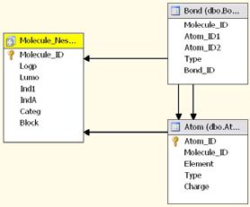
Database for DM (OLE DB DM) technology provides an industry standard for
developing DM algorithms [1]. This technology was first included in the
MSSQL 2000 release [2]. The MSSQL Analysis Services (SSAS) has included a
DM provider supporting two DM algorithms (one for classification by decision
trees and another for clustering) and the DM aggregator feature made possible
for developers and researchers to implement new DM algorithms. The MSSQL
2005 version [2] has included more seven algorithms as well as a new way to
aggregate new algorithms, using a plug-in approach instead of DM providers.
   Subscription       Participant
                                                        Company

                                                       Course

          Figure 1:     Registration – Four tables relational data.

      On the other hand, relational data impose some additional effort to deal
with them. While conventional classifiers assume that data sets are recorded in
single flat files or tables, a relational classifier has to face with more complex
data structures as shown by the simple Registration relational dataset [3]
represented by four tables in Fig. 1. In order to predict which participants are
going to attend a party, one needs participant personal data provided by table
Participant, participant employer data provided by table Company, participant
course subscriptions data provided by table Subscription and course data
provided by table Course.
      The usual approach to solve this problem is to use a single flat table, as
shown in Fig. 2, assembled by performing a relational join operation on the four
tables. But this approach may produce extremely large and impractical to handle
tables, with lots of repeated and null data.
      In consequence of those problems, multi-relational DM (MRDM)
approaches have been receiving considerable attention in the literature [3-11].
These approaches rely on developing specific algorithms to deal with the
relational feature of the data.
      By another way, OLE DB DM technology supports nested tables (also
known as table columns). As shown in Fig. 3, the row sets represent uniquely the
tables in a nested way. There are no redundant or null data for the participant in
each row set. One row per participant is all that is needed, and the nested
columns of the row set contain the data pertinent to that participant.
      In the next items, it will be presented a brief overview of the approaches
used to deal with MRDM, as well as the results of experiments carried out to
evaluate the scope of OLE DB DM approach. In these experiments the results of
MSDT algorithm are compared with those produced by TILDE [4]. Finally, the
conclusion is shown together with some recommendations to make
improvements in this field of research.
Figure 2: Registration – Unique table.
Name Job Company Type Party Course Length CourseType
erm 3 introductory
adams researcher scuf university yes so2 3 introductory
srw 3 advanced
srw 3 advanced
blake president jvt commercial yes
erm 3 introductory
srw 3 advanced
king manager ucro university yes erm 3 introductory
so2 3 introductory
martin manager ucro university yes
miller manager jvt commercial yes so2 3 introductory
porter researcher scuf university yes
cso 2 introductory
scott researcher scuf university no
abc 2 advanced
smith manager jvt commercial no cso 2 introductory
cso 2 introductory
turner researcher ucro university no
abc 2 advanced
Figure 3: Registration – Nested table.
2 Multi-relational DM approaches
2.1 Unique table approach
Most classifiers works on a single table (attribute-value learning) with a fixed set
of attributes. So it is restrictive in DM applications with multiple tables. It ispossible to construct, by hand, a single table by performing a relational join
operation on multiple tables using propositional logic as shown in Fig. 2.
For one-to-one and many-to-one relationships, one can join in the extra
fields to the original relation without problems. For one to many relationships,
there are two ways to handle them. The first one is just compute the join, but this
leads to data redundancy, missing values, statistical skew, and loss of meaning.
A single instance in the original database is mapped onto multiple instances in
the new table, which is problematic. The second way is aggregate the
information in different tuples representing the same individual into one tuple
after computing the join. This removes the problems mentioned above, but
causes loss of information because details originally present have been
summarized away.
2.2 Multi-relational DM algorithms
This is a group of several approaches [5]: Propositional Learning; Inductive
Logic Programming (ILP); Multi-Relational DM (MRDM); First Order Bayesian
Networks (FOBN).
The Propositional Learning approach is a two independent step process, in
which the initial one produces automatically a flat table that can be processed in
the second step by any DM algorithm. It is essentially the same as described in
the unique table approach, and has the same problems.
The ILP [3,4,7] approaches handle multiple tables directly, using a first
order logic language to describe patterns extending over multiple tuples. These
approaches include: Progol, First Order Inductive Logic (FOIL), TILDE [4],
Inductive Constraint Logic (ICL), and CrossMine [8].
The MRDM approaches include a number of variants such as those
presented by the following studies: Multi-Relational Decision Tree Induction [9],
Multi-Relational Decision Tree (MRDT) [5], Multi-Relational Naïve Bayes
Classifier (Mr-SBC) [10], and Multi-Relational Model Trees with support to
regression (Mr-SMOTI) [11]. They do essentially the same as the IPL
approaches do, but work in the relational database setting.
Finally, FOBN approaches extend the ILP or MRDM approaches by
combining them with probabilistic (Bayesian) reasoning. These approaches
include: Probabilistic Relational Model (PRM) [12], Probabilistic Logic Program
(PLP), Bayesian Logic Program (BLP), and Stochastic Logic Program (SLP).
2.3 OLE DB DM nested tables
MS OLE DB DM uses nested DM columns (nested tables). DM models (DMMs)
use this nested column structure for both input and output data, as the syntax
used to populate a DMM with training data allows nested columns to be
represented as sub-queries. DM algorithms cannot work directly with this
approach. Unnesting them using the traditional unnest operator yields a single
table in the same format as the join approach mentioned above, with the same
problems. To avoid these problems is used a sparse matricial approach.
First of all are produced expanded versions of the main (case and nested)tables by joining them on their support tables. Support tables are those that the
main tables holds one-to-one or many-to-one relationship with them. The lines of
this matrix are the expanded case table records and the matrix columns are the
compound attributes. These compound attributes are the expanded case table
normal attributes plus additional attributes that correspond to all elements of the
expanded nested tables mapped by columns.
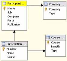
To exemplify this approach the relational Registration DMM shown in
Fig. 4 will be used. The Company support table is joined with Participant case
table to produce its expanded version, addind more one attribute
(CompanyType) to the original main table. The join of Subscription nested
table with Course support table adds more two attributes (Lenght and Type) to
the nested table producing its expanded version.
Figure 4: Registration - DMM schema. Participant is the
case table, Subscription is the nested table and
Course and Company are the support tables.
Attributte number/attribute name
0 1 2 3
Num of
Num Case Party Company Job CompanyType
attributes
1 1:adams 16 2:yes 2:scuf 3:researcher 2: university
2 2:blake 12 2:yes 1:jvt 2:president 1:commercial
3 3:king 16 2:yes 3:ucro 1:manager 3: university (2:)
4 martin 4 2:yes 3:ucro 1:manager 3: university (2:)
5 4:miller 8 2:yes 1:jvt 1:manager 1:commercial
6 porter 4 2:yes 2:scuf 3:researcher 2: university
7 5:scott 12 1:no 2:scuf 3:researcher 2: university
8 6:smith 8 1:no 1:jvt 1:manager 1:commercial
9 7:turner 12 1:no 3:ucro 3:researcher 3: university (2:)
Figure 5: Registration – Sparse matrix normal attributes
The Registration sparse matrix has nine lines (the dataset cases) and sixty
attributes. Four of them are the normal attributes (Fig. 5) and fifty six are the
additional attributes mapped from the columns of the expanded nested table (Fig.
6). These fifty six attributes correspond to the fourteen records times the fourattributes of the Subscription expanded nested table. The name of each
additional attribute is composed by the name of the nested table plus the name
(or number) of its key attribute (ID) plus the name of the attribute considered as
it can be seen in Fig. 6. Some problems with attribute values could be observed.
In Fig. 5 the CompanyType attribute must have only two different values but
three values were retrieved from the dataset. This same behaviour was observed
in several others attributes as it can be seen in Fig. 6. The reason for this
unexpected behaviour is not clear to us.
Attributte number/attribute name
4 5 6 7 8 9 10 11 12 13 14 15 16 17 18 19 20 21 22 23 24 25 26 27 28 29 30 31
Sub Sub Sub Sub Sub Sub Sub Sub Sub Sub Sub Sub Sub Sub Sub Sub Sub Sub Sub
Subs Sub Sub Sub Sub Sub Sub Sub Sub
scrip scrip scrip scrip scrip scrip scrip scrip scrip scrip scrip scrip scrip scrip scrip scrip scrip scrip scrip
cripti scrip scrip scrip scrip scrip scrip scrip scrip
tion( tion( tion( tion( tion( tion( tion( tion( tion( tion( tion( tion( tion( tion( tion( tion( tion( tion( tion(
Num on(1) tion( tion( tion( tion( tion( tion( tion( tion(
10). 11). 12). 13). 14). 1).C 2).C 3).C 4).C 5).C 6).C 7).C 8).C 9).C 10). 11). 12). 13). 14).
.Nam 2).N 3).N 4).N 5).N 6).N 7).N 8).N 9).N
Nam Nam Nam Nam Nam ours ours ours ours ours ours ours ours ours Cou Cou Cou Cou Cour
e ame ame ame ame ame ame ame ame
e e e e e e e e e e e e e e rse rse rse rse se
1:ada 1:ad 1:ad 3:er 4:so 5:sr
1
ms ams ams m 2 w
2: 2:
5:sr 3:er
2 blak blak
w m
e e
3:kin 3:kin 3:kin 5:sr 3:er 4:so
3
g g g w m 2
4
4:mil 4:so
5
ler 2
6
5:sc 5:sc 2:cs 1:ab
7
ott ott o c
6:sm 2:cs
8
ith o
7:tur 7:tur 2:cs 1:ab
9
ner ner o c
Attributte number/attribute name
32 33 34 35 36 37 38 39 40 41 42 43 44 45 46 47 48 49 50 51 52 53 54 55 56 57 58 59
Sub Sub Sub Sub Sub Sub Sub Sub Sub Sub Sub Sub Sub Sub
Sub Sub Sub Sub Sub Sub Sub Sub Sub Sub Sub Sub Sub Sub
scrip scrip scrip scrip scrip scrip scrip scrip scrip scrip scrip scrip scrip scrip
scrip scrip scrip scrip scrip scrip scrip scrip scrip scrip scrip scrip scrip scrip
tion( tion( tion( tion( tion( tion( tion( tion( tion( tion( tion( tion( tion( tion(
tion( tion( tion( tion( tion( tion( tion( tion( tion( tion( tion( tion( tion( tion(
Num 1).C 2).C 3).C 4).C 5).C 6).C 7).C 8).C 9).C 10). 11). 12). 13). 14).
1).L 2).L 3).L 4).L 5).L 6).L 7).L 8).L 9).L 10). 11). 12). 13). 14).
ours ours ours ours ours ours ours ours ours Cou Cou Cou Cou Cour
engt engt engt engt engt engt engt engt engt Len Len Len Len Len
eTy eTy eTy eTy eTy eTy eTy eTy eTy rseT rseT rseT rseT seTy
h h h h h h h h h gth gth gth gth gth
pe pe pe pe pe pe pe pe pe ype ype ype ype pe
3:int 4:int 5:ad
3:3 4:3 5:3 rodu rodu vanc
1
(2:) (2:) (2:) ctor ctor ed
y (2:) y (2:) (1:)
5:ad 3:int
5:3 3:3 vanc rodu
2
(2:) (2:) ed ctor
(1:) y (2:)
5:ad 3:int 4:int
5:3 3:3 4:3 vanc rodu rodu
3
(2:) (2:) (2:) ed ctor ctor
(1:) y (2:) y (2:)
4
4:int
4:3 rodu
5
(2:) ctor
y (2:)
6
2:int
1:ad
2:2 rodu
7 1:2 vanc
(1:) ctor
ed
y
2:int
2:2 rodu
8
(1:) ctor
y
2:int
1:ad
2:2 rodu
9 1:2 vanc
(1:) ctor
ed
y
Figure 6: Registration – Sparse matrix additional attributes.
3 Computational Experiments
Two experiments were carried out in order to evaluate the scope of MSSQL
while dealing with MRDM. Two datasets are used: Registration [3] and
Mutagenesis [13]. The numeric results and the decision trees obtained by MSDT
(using the sparse matrix) in these experiments were compared with those
produced by TILDE (using the original data). These experiments were made by
using an IBM PC compatible microcomputer, Intel Pentium M 2.00 GHz
processor inside, 1.0 GB of RAM memory, 1.5 GB virtual memory, 100 MB
hard disk, MS Windows XP Pro SP2 and MSSQL 2005 Enterprise installed.3.1 Registration dataset
Figure 7: Registration – MSDT Decision tree.
subscription(-A),course_len(A,2) ?
+--yes: [party_no] 3.0 [[party_yes:0.0,party_no:3.0]]
+--no: [party_yes] 6.0 [[party_yes:6.0,party_no:0.0]]
Figure 8: Registration – TILDE Decision tree.
Both MSDT and TILDE achieved full accuracy while training this dataset and
using itself as the test dataset. TILDE showed a meaningful decision tree (Fig.
8), stating that a participant attends the party if he or she has a subscription to a
course of length 2, while MDST showed attributes in its decision tree (Fig. 7)
that are difficult to interpret, e.g., subscription(9).Name not= missing has no real
meaning because the subscription numbering is not defined globally.
3.2 Mutagenesis dataset
This dataset concerns with the problem of identifying the mutagenic compounds
and have been extensively used to test both ILP and MRDM systems. It was
considered, analogously to related experiments in the literature, the regression
friendly dataset of 188 elements. It was used the background knowledge BK2,
which consists of those data obtained with the modelling package Quanta, plus
indicators ind1, indA and attributes logp and lumo [11]. Only two classes were
considered for the prediction attribute: positive or negative. We used ten-fold
cross-validation to estimate the accuracy of the classifiers. The DMM schema is
shown in Fig. 9. Some parameters were the same for both MSDT1 and MSDT2:
COMPLEXITY_PENALTY = 0.1, MAXIMUM_INPUT_ATTRIBUTES = 255,
MAXIMUM_OUTPUT_ATTRIBUTES = 255, SCORE_METHOD = 4 and
SPLIT_METHOD = 3. MSDT1 uses MINIMUM_SUPPORT = 10 and MSDT2
uses MINIMUM_SUPPORT = 1. MSDT1 configuration uses all input attributes
and MSDT2 uses only Atom and Bond input attributes.Figure 9: Mutagenesis – DMM schema.
Figure 10: Mutagenesis – MSDT1 Decision Tree.
Figure 11: Mutagenesis – MSDT2 Decision Tree.
MSDT1 achieved 87±6% of accuracy while MSDT2 got 66±13% (because
the Molecule input attributes were deliberately ignored). TILDE got 80±3% of
accuracy. Figs. 10 to 12 show one of the ten-fold cross validation decision trees
produced by the corresponding classifiers. TILDE showed a meaningful decision
tree (Fig. 12) compared with those produced by MDST (Fig. 10 and 11). By
example, tests such as atom(d104_38).Type not = missing (Fig. 11) are notinterpretable because there is no natural numbering for the atoms. This illustrates
the loss of meaning: atom #n has a meaning in the current representation of the
data (it is the n'th atom in our ordered list), but not in the real world (because the
atoms in a molecule are not actually ordered). Multi-relational trees, of which the
TILDE trees shown in Fig. 12 are an example, avoid this problem: they refer to
atoms not with some specific ID (e.g., d104_38) but through variables and
properties of these (e.g., a C-atom of type 35) that always have meaning. That is
the crucial difference between the MSDT trees shown here, and multi-relational
trees.
For this dataset it was produced a sparse matrix with 188 cases and 23,996
attributes. Five of them are the normal attributes, 6,309 for Bond(i).Type and
17,682 for Atom(j).Element, Atom(j).Charge and Atom(j).Type (3*5894). For
huge datasets with several nested tables it suggests an explosion on the number
of additional attributes that can be unfeasible to handle.
dmuta(-A,-B)
atom(A,-C,-D,27,-E) ?
+--yes: atom(A,-F,-G,35,-H) ?
| +--yes: [neg] 7.0 [[neg:6.0,pos:1.0]]
| +--no: [pos] 67.0 [[neg:5.0,pos:62.0]]
+--no: atom(A,-I,-J,29,-K) ?
+--yes: atom(A,-L,-M,1,-N) ?
| +--yes: atom(A,-O,-P,10,-Q) ?
| | +--yes: [pos] 3.0 [[neg:0.0,pos:3.0]]
| | +--no: [neg] 8.0 [[neg:6.0,pos:2.0]]
| +--no: [pos] 30.0 [[neg:5.0,pos:25.0]]
+--no: atom(A,-R,-S,52,-T) ?
+--yes: [pos] 2.0 [[neg:0.0,pos:2.0]]
+--no: [neg] 52.0 [[neg:33.0,pos:19.0]]
Figure 12: Mutagenesis – TILDE Decision tree.
4 Conclusion and future work
MSDT showed very good results when using only attributes of the target table,
but it seems it cannot handle information in nested tables in a meaningful way:
trees thus produced are meaningless and tend to obtain poor predictive accuracy
on unseen data. There are, however, a number of questions still unanswered
with respect to the plug-in framework of MS SQL and the use of MSDT
approach in this framework. In particular, it is unclear what the best approach
would be to implement a truly relational algorithm in this framework.
We are running more experiments to better understand the plug-in
framework and furthermore we are investigating which algorithm could be the
more suitable to be implemented in this framework.
In the experiments we perform, MSDT has equally and even better good
predictive accuracy as TILDE, but the trees it gives either ignore the relational
information, or use it in a way that yields non-interpretable trees. As such, one
could say that its explanatory power is reduced, when compared to a multi-
relational decision tree learner.Finally we conclude that would be useful to integrate multi-relational
learners into MSSQL and we are proposing to implement such kind of algorithm
to deal with relational DM and to achieve database mining integration.
5 Acknowledgments
Claudio L. Curotto is a post-doctoral fellow of the National Council for
Scientific and Technological Development (CNPq) and Hendrik Blockeel is a
post-doctoral fellow of the Fund for Scientific Research of Flanders, Belgium.
References
[1] Microsoft Corporation, OLE DB for Data Mining Specification 1.0 Final,
2000 http://www.microsoft.com/downloads/details.aspx?displaylang=en&fa
milyid=01005f92-dba1-4fa4-8ba0-af6a19d30217.
[2] Microsoft Corporation, SQL Server Home http://www.microsoft.com/sql/.
[3] Dzeroski, S. & Lavrac, N. (eds.), Relational Data Mining, Springer, Berlin,
Germany, 2001.
[4] Blockeel, H., Top-down induction of first order logical decision trees, Ph.D.
thesis, Department of Computer Science, Katholieke Universiteit Leuven,
Leuven, Belgium, 1998.
[5] Leiva, H.A., MRDTL: A Multi-Relational Decision Tree Learning
Algorithm, M.Sc. Thesis, Iowa State University, Ames, Iowa, USA, 2002.
[6] Knobbe, A.J., Haas, M. de & Siebes, A., Propositionalization and
Aggregates, in Proc. of the PKDD 2001, Springer, Berlin, Germany, pp 277-
288, 2001.
[7] Dzeroski, S. et alli, Summer School on Relational Data Mining 2002,
http://www-ai.ijs.si/SasoDzeroski/RDMSchool.
[8] Yin, X., Han, J. & Yang, J., Efficient Multi-Relational Classification by
Tuple ID Propagation, in Proc. of the 2nd MRDM Workshop, 2003.
[9] Knobbe, A.J., Siebes, A. & Van der Wallen, D.M.G., Multi-Relational
Decision Tree Induction, in Proc. of the PKDD’99, Springer, Berlin,
Germany, pp 378-383, 1999.
[10] Ceci, M., Appice, A. & Malerba, D., Mr-SBC: a Multi-Relational Naive
Bayes Classifier, in PKDD 2003, Lecture Notes in Artificial Intelligence
2838, Lavrac, N., Gamberger, D., Todorovski, L. & Blockeel, H. (eds.),
Springer, Berlin, Germany, pp. 95-106, 2003.
[11] Appice, A., Ceci, M. & Malerba, D., Mining Model Trees: A Multi-
Relational Approach, in ILP'03, Lecture Notes in Artificial Intelligence
2835, Horvath, T. and Yamamoto, A. (eds.), Springer, Berlin, Germany, pp
4-21, 2003.
[12] Getoor, L., Learning Statistical Models from Relational Data, Ph.D. Thesis,
Stanford University, Stanford, California, USA, 2001.
[13] Muggleton, S.H., Inductive Logic Programming web site - Predicting
mutagenicity http://www.doc.ic.ac.uk/~shm/mutagenesis.html.You can also read