Multi-source cross-project software defect prediction based on deep integration

Journal of Physics: Conference Series

PAPER • OPEN ACCESS

Multi-source cross-project software defect prediction based on deep
integration
To cite this article: Jing Zhang et al 2021 J. Phys.: Conf. Ser. 1861 012075

View the article online for updates and enhancements.

 This content was downloaded from IP address 46.4.80.155 on 21/09/2021 at 11:19

IWAACE 2021 IOP Publishing
Journal of Physics: Conference Series 1861 (2021) 012075 doi:10.1088/1742-6596/1861/1/012075

Multi-source cross-project software defect prediction based on
deep integration

 Jing Zhang1, Wei Wang1∗, Yun He2, Xinfa Li1
 1
 Department of software Engineering, Yunnan University, Yunnan 650504, China
 2
 Department of software Engineering, Yunnan Agricultural University, Yunnan
 650504, China
 wangwei@ynu.edu.cn

 Abstract. Cross-project defect prediction (CPDP), training a machine learning model by using
 training data from other projects, has attracted much attention in recent years. This approach
 provides a feasible way for small-scale or new developed project with insufficient training data
 to carry out defect prediction. This paper focus on the bottleneck issue of CPDP, poor accuracy,
 and propose a deep learning model integration-based approach (MTrADL) for CPDP. This paper
 consists of two main phases. First, the similarity between target project and source projects is
 measured by the modified maximum mean discrepancy (MMD) and the top K source projects
 with high similarity to the target project are selected as training data. Second, for the selected
 training data, this paper use convolutional neural network (CNN) to build the defect predictor.
 Each selected training data corresponds to one CNN predictor. Then, multiple predictors are
 integrated to get the final prediction result. To examine the performance of the proposed
 approach, this paper conduct experiments on 41 datasets of PROMISE and compare our
 approach with three state-of-the-art baseline approaches: a training data selection model (TDS),
 a two-stage transfer learning model (TPTL), and the multi-source transfer learning model
 (MTrA). The experimental results show that the average F1-score of our approach is 0.76. Across
 the 41 datasets, on average, MTrADL respectively improves these baseline models by 39.8%,
 28.50%, and 10% in terms of F1-score.

1. Introduction
The purpose of software defect prediction [1, 2] is to predict the number and distribution of software
defects. Predicting results is of great significance for optimizing test resource allocation and reducing
maintenance costs [3, 4]. Most existing approaches followed the cross-project defect prediction (CPDP)
[5-10], which use training data from other projects (called source projects) to build the predictor for the
project to be analyzed (called target project). Briand et al. [11] proposed the first CPDP model in 2002.
Their experimental results showed the feasibility and potential usefulness of CPDP.
 In order to improve the performance, two feasible ways are introduced [11, 12] (1) selecting
appropriate source projects and (2) developing innovative defect modeling method.
 In this study, we propose a multi-source cross-project defect prediction approach (MTrADL) based
on deep learning. First, the modified maximum mean discrepancy (MMD) is used to select the source
projects. Second, the convolutional neural network (CNN) is used as the base learner to build the defect
predictor. Third, the final prediction result is generated by predictors integration.

 Content from this work may be used under the terms of the Creative Commons Attribution 3.0 licence. Any further distribution
 of this work must maintain attribution to the author(s) and the title of the work, journal citation and DOI.
Published under licence by IOP Publishing Ltd 1

IWAACE 2021 IOP Publishing
Journal of Physics: Conference Series 1861 (2021) 012075 doi:10.1088/1742-6596/1861/1/012075

2. Proposed approach
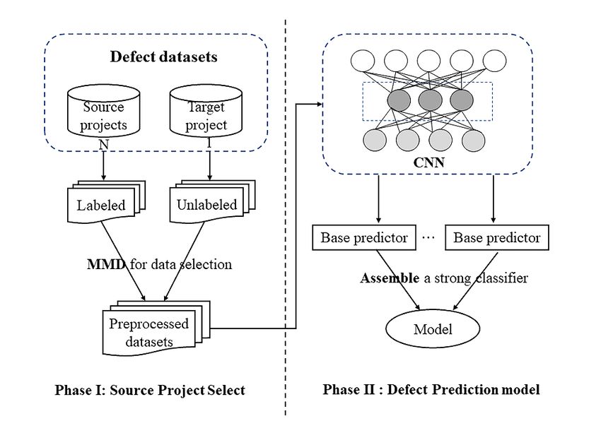
As shown in Figure.1, in order to improve the prediction accuracy of CPDP, we proposed MTrADL
which involves two phases: source project selection and defect prediction model construction and
integration.
 In the first phase, MMD is used to evaluate the similarity between the multiple source projects and
target project. The projects with the top k high similarity to the target project are selected as the training
data to build the defect prediction model. In the second phase, each selected training data corresponds
to one CNN predictor. Then the final predicting result is generated by integrating multiple predictors
together.
 In this section, it is supposed that we have N source projects { 1 , 2 , … , } and a target project T.
Each source project contains many instances, and each instance corresponds to a class. Every instance
involves two parts: a set of metrics x and its corresponding label y that is used to indicate the defective
status (y=1 indicates defective, y=0 indicates clean). The purpose of MTrADL is to predict the
corresponding label of one instance in the future by using the model trained with source projects
{ 1 , 2 , … , } and the target project T.

 Figure.1 Process of MTrADL for CPDP

2.1 Source project selection
The source project selection aims to select K dataset from N candidate source datasets ( ≤ ), to build
the training dataset for predictor.
 In this subsection, we propose the source projects selection process based on the modified max mean
discrepancy (MMD) [13, 14], and the similarity between source and target datasets is reflected as the
similarity index. Then the source datasets s = { 1 , 2 , … , } are ranked by the similarity and the top K
source datasets are selected as the training data for the predictor.
 As shown in equation 1, MMD uses kernel function ϕ(∙) to map linear inseparable data into the
reproducing kernel hilbert space (RKHS) to make it linearly separable. The distance between the center
points of two datasets is used to characterized the probability distribution difference between such two
datasets. Here, xt,i and xs,i refer to the ith data of the target change data set and the source change data
set, while nt and ns represent the number of target data and source data, respectively.
 2
 nt ns
 1 1
 MMD( X t , X s ) =
 nt
 
 i =1
  ( xt ,i ) −
 ns
  ( x
 i =1
 s ,i )
  (1)
 However, we believe that the distance between center points of two dataset just reflects the difference
from the perspective of mean. The variance is also an important characteristic for depicting the

 2

IWAACE 2021 IOP Publishing
Journal of Physics: Conference Series 1861 (2021) 012075 doi:10.1088/1742-6596/1861/1/012075

probability distribution difference. Because of the distribution of the two data varies greatly due to the
big variance difference. Therefore, we define the variance difference between two linearly separable
datasets in RKHS as follows:
 2 2 2
 1 
 nt
 1 nt
  1 ns
  1 ns
 
 Var =    ( xt ,i )-   ( xt ,i )  − n    ( xs ,i )- n   ( xs , i ) 
 nt i =1  nt i =1  s i =1  s i =1 
 (2) 

 The modified MMD (MVMD) is defined as follows. The is a hyperparameters defined by the
users, which reflects the relative importance of such two factors.
 MVMD( X s , X t ) = Var + (1 −  ) MMD (3)
 MMD is used to evaluate the similarity between the multiple source projects and the target project.
Furthermore, according to the He et al. [15], recommendation the number of source projects should not
exceed, we adopt this suggestion here and set the K equal to 3. Each project selected is called a dataset.

2.2 Defect prediction model construction and integration
In this section, we focus on CNN’s powerful ability of capturing highly complicated non-linear features
as the base learner for each selected source dataset [16].
 We trained CNN with the training data selected in the previous phase. CNN is just an application of
this research, so we adopt the standard CNN architecture to build our base predictor [17].

 Figure.2 Construction process of CNN model

 As shown in Figure.2, other details of the CNN are as follows:
 1. Input Layer: Through the data selection process described in the previous section, K source
projects and a target project are obtained as the training datasets.
 2. Convolutional layers: Researchers generally believe that adding depth of a model can achieve
better results. Therefore, in this paper, we increase the number of convolutional layers from 1 to 2.
 3. Activation function: Using the sigmoid activation function for classification.
 4. Training and optimizer: Using an Adam optimizer [18] to train our model, which makes training
faster.
 Using the idea of deep learning, training method of CPDP based on instance migration is adopted.
According to the above-mentioned steps, K base predictors suitable for the target project can be trained,
and CPDP can be conducted for the target dataset.
 Then used the K base predictors to generate final predicting result with the help of one ensemble
learning technique.

3. Experiment
In order to evaluate the properties of proposed approach, the datasets, experimental design ,experimental
results are presented in this section.

 3

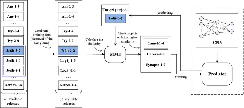
IWAACE 2021 IOP Publishing
Journal of Physics: Conference Series 1861 (2021) 012075 doi:10.1088/1742-6596/1861/1/012075

3.1 Datasets
As shown in Table 1, the defect datasets used in this paper are collected by Jureczko and Madeyski from
PROMISE data warehouse [19].
 The datasets contain 71 releases of 38 different open source software projects and 6 releases of
proprietary projects. In this experiment, as shown in Table 1, we used the same data set as that used by
Liu and discarded releases ckjm. Table 1 lists the defect datasets (including data category and total
number of defects) of the 41 releases from 14 software projects that we used.
 Data preprocessing. Preprocessing involves two steps: normalization and imbalanced data handling.
We transform all values of metrics into the [0,1] and use SMOTE to perform class imbalance processing
such that the existing binary label had a positive to negative ratio of 5:5.

 Table1. Datasets
 Dataset #Class #Defect（%） #Target Data set #Class #Defect（%） #Target
 ant-1-3 125 20（16.00%） 36 lucene-2-2 247 144（58.30%） 38
 ant-1-4 178 40（22.47%） 36 lucene-2-4 340 203（59.71%） 38
 ant-1-5 293 32（10.92%） 36 poi-1-5 237 141（59.49%） 37
 ant-1-6 351 92（26.21%） 36 poi-2-0 314 37（11.78%） 37
 ant-1-7 745 166（22.28%） 36 poi-2-5 385 248（64.42%） 37
 camel-1.0 339 13（3.83%） 37 poi-3-0 442 281（63.57%） 37
 camel-1.2 608 216（35.53%） 37 redactor 176 27（15.34%） 40
 camel-1.4 872 145（16.63%） 37 synapse-1-0 157 16（10.19%） 38
 camel-1.6 965 188（19.48%） 37 synapse-1-1 222 60（27.03%） 38
 ivy-1.1 111 63（56.76%） 38 synapse-1-2 256 86（33.59%） 38
 ivy-1.4 241 16（6.64%） 38 tomcat 858 77（8.97%） 40
 ivy-2.0 352 40（11.36%） 38 velocity-1-4 196 147（75.00%） 39
 jedit-3.2 272 90（33.09%） 36 velocity-1-6 229 78（34.06%） 39
 jedit-4.0 306 75（24.51%） 36 xalan-2-4 723 110（15.21%） 37
 jedit-4.1 312 79（25.32%） 36 xalan-2-5 803 387（48.19%） 37
 jedit-4.2 367 48（13.08%） 36 xalan-2-6 885 411（46.44%） 37
 jedit-4.3 492 11（2.24%） 36 xalan-2-7 909 898（98.79%） 37
 log4j-1-0 135 34（25.19%） 38 xerces-1-2 440 71（16.14%） 38
 log4j-1-1 109 37（33.94%） 38 xerces-1-3 453 69（15.23%） 38
 log4j-1-2 205 189（92.20%） 38 xerces-1-4 588 437（74.32%） 38
 lucene-2-0 195 91（46.67%） 38

3.2 Experimental design
We choose one release of a project as target dataset, and the remaining 13 projects were used as
candidate source datasets.

 Figure.3 Framework of our approach: an example of the target project jedit-3-2

 If the target project contained multiple releases, we keep on one release and other releases are
removed, and all releases of the remaining projects were used as the candidate source datasets for the
experiments. Figure.3 presents an example of the experimental setup of the MTrADL method, when

 4

IWAACE 2021 IOP Publishing
Journal of Physics: Conference Series 1861 (2021) 012075 doi:10.1088/1742-6596/1861/1/012075

release jedit-3-2 is used as the target dataset, the releases jedit-4-0, jedit-4-1, jedit-4-2, and jedit-4-3 are
removed. All remaining 13 projects are used as candidate source datasets.
 Baseline Methods. In order the show the feasibility and the advance nature of our approach, we tried
to find out how effective it is in CPDP and whether it can perform better than the baseline methods. The
TPTL [20], TDS [6] and MTrA [21] are set as the baseline methods.

4. Results and discussion
In this section, we discuss our experimental results and answer the research questions raised in the
previous section.
 F1-score comparison of MTrADL model and three baseline models (TDS, TPTL, and MTrA) for 41
datasets. “W/T/L” denotes the number of data sets when the baseline model performs better than
MTrADL, when the baseline model performs as well as MTrADL, and when the baseline model
performs worse than MTrADL, respectively.
 Table 2.F1-score comparison of MTrADL model and three baseline models
 Datasets 1. TDS 2.TPTL 3.MTrA 4.OUR
 APPROACH
 ant-1-3 0.394 0.456 0.721 0.827
 ant-1-4 0.345 0.377 0.571 0.778
 ant-1-5 0.262 0.237 0.690 0.779
 ant-1-6 0.449 0.595 0.746 0.827
 ant-1-7 0.454 0.455 0.709 0.789
 camel-1-0 0.111 0.093 0.752 0.843
 camel-1-2 0.378 0.502 0.684 0.865
 camel-1-4 0.323 0.339 0.623 0.659
 camel-1-6 0.190 0.356 0.657 0.723
 ivy-1-1 0.642 0.738 0.596 0.667
 ivy-1-4 0.000 0.160 0.333 0.813
 ivy-2-0 0.305 0.349 0.744 0.778
 jedit-3-2 0.143 0.536 0.633 0.800
 jedit-4-0 0.235 0.447 0.713 0.831
 jedit-4-1 0.239 0.522 0.728 0.763
 jedit-4-2 0.440 0.370 0.736 0.838
 jedit-4-3 0.112 0.050 0.776 0.926
 log4j-1-0 0.528 0.637 0.756 0.800
 log4j-1-1 0.538 0.699 0.613 0.737
 log4j-1-2 0.314 0.606 0.661 0.649
 lucene-2-0 0.542 0.677 0.568 0.625
 lucene-2-2 0.581 0.621 0.707 0.605
 lucene-2-4 0.700 0.633 0.738 0.627
 poi-1-5 0.600 0.713 0.723 0.632
 poi-2-0 0.217 0.218 0.716 0.705
 poi-2-5 0.554 0.728 0.715 0.756
 poi-3-0 0.699 0.787 0.654 0.681
 redactor 0.304 0.353 0.678 0.750
 synapse-1-0 0.526 0.253 0.643 0.824
 synapse-1-1 0.487 0.475 0.647 0.773
 synapse-1-2 0.510 0.571 0.676 0.659
 tomcat 0.083 0.287 0.684 0.835
 velocity-1-4 0.136 0.734 0.736 0.830
 velocity-1-6 0.025 0.568 0.738 0.717
 xalan-2-4 0.345 0.403 0.761 0.861

 5

IWAACE 2021 IOP Publishing
Journal of Physics: Conference Series 1861 (2021) 012075 doi:10.1088/1742-6596/1861/1/012075

 xalan-2-5 0.448 0.533 0.598 0.574
 xalan-2-6 0.647 0.512 0.632 0.679
 xalan-2-7 0.345 0.616 0.011 0.943
 xerces-1-2 0.167 0.192 0.612 0.684
 xerces-1-3 0.256 0.377 0.712 0.869
 xerces-1-4 0.250 0.690 0.664 0.826
 Average 0.362 0.475 0.660 0.760
 Improved Compared with Compared Compared with —
 No.4 with No.4 No.4
 ↓39.80 % ↓28.50 % ↓10.00 % —
 W/T/L 2/0/39 6/0/35 8/0/33 —

 Prediction performance. In terms of F1-score, the average values vary from 0.362, 0.475, 0.660 to
0.760 by using TDS, TPTL, MTrA, and MTrADL respectively.
 Compared with TDS, MTrADL can achieve better performance on average. In terms of F1-score,
MTrADL has 39.80% improvement as shown in Table 2. Therefore, it can be concluded that MTrADL
has significant improvement than TDS in the performance of the F1-score. Especially, MTrADL can
achieve the most significant improvements on releases camel-1-0, jedit-3-2, jedit-4-3, velocity-1-4, and
xerces-1-2.
 Compared with TPTL, MTrADL can achieve better performance on average. In terms of F1-score,
MTrADL has 28.50% improvement as shown in Table 2. Therefore, it can be concluded that MTrADL
has significant improvement than TPTL in the performance of the F1-score. Especially, MTrADL can
achieve the most significant improvements on releases ivy-1-4 and camel-1-0.
 Compared with MTrA, MTrADL can achieve better performance on average. In terms of F1-score,
MTrADL has 10% improvement as shown in Table 2. Therefore, it can be concluded that MTrADL has
significant improvement than MTrA in the performance of the F1-score.
 Number of improvements. The statistical test showed that MTrADL outperforms TDS, TPTL, and
MTrA on 39, 35 and 33 datasets, respectively, and the improvement rate exceeds 80.49%. Hereinafter
to be referred as numbers. Thus, our approach achieved significant improvements in data selection and
multi-source defect prediction.

5. Conclusion
This paper proposed a multi-source transfer learning model, namely MTrADL, based on deep learning
for CPDP. The MTrADL model is highly effective, with an improvement rate of over 80.49%.
 (1) From the perspective of predictive performance, compared to TDS and TPTL, the average F1-
score improved by 39.8% and 28.50%, respectively. Compared with the classical MTrA algorithm, the
average F1-score improved by 10%.
 (2) From the perspective of the number of datasets, MTrADL outperformed TDS, TPTL, and MTrA
on 39, 35, and 33 datasets, respectively, with an improvement rate of over 80.49%.

Acknowledgments
This work was supported by the National Natural Science Foundation of China under Grant Nos.
61462092, 61379032, and 61662085, the Young Scientist Scholarship of the Chinese Academy of
Sciences under Grant No. W8090311, and the Scientific Research Fund project of Yunnan Education
Department under Grant Nos. 2020Y0005 and 2020J0239.

References
[1] B. Caglayan, A. T. Misirli ,et al. Predicting defective modules in different test phases[J]. Software
 Quality Journal, 2015,23(2): 205-227.
[2] Y. CHEN, X.-h. SHEN ,et al. Application of Probabilistic Relational Model to Aerospace Software
 Defect Prediction[J]. Optics and Precision Engineering, 2013,21(7): 1865-1872(in Chinese).

 6

IWAACE 2021 IOP Publishing
Journal of Physics: Conference Series 1861 (2021) 012075 doi:10.1088/1742-6596/1861/1/012075

[3] S. Hosseini, B. Turhan ,et al. A systematic literature review and meta-analysis on cross project defect
 prediction[J]. IEEE Transactions on Software Engineering, 2017,45(2): 111-147.
[4] X. Xia, E. Shihab ,et al. "Predicting crashing releases of mobile applications," in Proceedings of the
 10th ACM/IEEE International Symposium on Empirical Software Engineering and
 Measurement, 2016:1-10(in Chinese).
[5] P. He, B. Li ,et al. Simplification of training data for cross-project defect prediction[J]. arXiv preprint
 arXiv:1405.0773, 2014(in Chinese).
[6] S. Herbold. "Training data selection for cross-project defect prediction," in Proceedings of the 9th
 International Conference on Predictive Models in Software Engineering, 2013.
[7] S. Amasaki, K. Kawata ,et al. "Improving cross-project defect prediction methods with data
 simplification," in 2015 41st Euromicro Conference on Software Engineering and Advanced
 Applications, 2015:96-103.
[8] Y. Li, Z. Huang ,et al. Evaluating data filter on cross-project defect prediction: Comparison and
 improvements[J]. IEEE Access, 2017,5:25646-25656(in Chinese).
[9] F. Rahman, D. Posnett ,et al. "Recalling the imprecision of cross-project defect prediction," in
 Proceedings of the ACM SIGSOFT 20th International Symposium on the Foundations of
 Software Engineering, 2012:61.
[10] W. Wen, B. Zhang ,et al. "An Empirical Study on Combining Source Selection and Transfer
 Learning for Cross-Project Defect Prediction," in 2019 IEEE 1st International Workshop on
 Intelligent Bug Fixing (IBF), 2019:29-38(in Chinese).
[11] L. C. Briand, W. L. Melo ,et al. Assessing the applicability of fault-proneness models across
 object-oriented software projects[J]. IEEE transactions on Software Engineering, 2002,28(7):
 706-720.
[12] T. Zimmermann, N. Nagappan ,et al. "Cross-project defect prediction: a large scale experiment
 on data vs. domain vs. process," [J]. the 7th joint meeting of the European software engineering
 conference, 2009:91-100.
[13] A. Gretton, K. M. Borgwardt ,et al. A kernel two-sample test[J]. Journal of Machine Learning
 Research, 2012,13(Mar): 723-773.
[14] A. Smola, A. Gretton ,et al. "A Hilbert space embedding for distributions," in International
 Conference on Algorithmic Learning Theory, 2007:13-31.
[15] Z. He, F. Shu ,et al. An investigation on the feasibility of cross-project defect prediction[J].
 Automated Software Engineering, 2012,19(2): 167-199(in Chinese).
[16] Pan, Lu ,et al. An Improved CNN Model for Within-Project Software Defect Prediction[J].
 Applied Sciences, 2019,9(10): 21-38(in Chinese).
[17] A. Krizhevsky, I. Sutskever ,et al. "Imagenet classification with deep convolutional neural
 networks," in Advances in neural information processing systems, 2012:1097-1105.
[18] D. Kingma, and J. Ba. Adam: A Method for Stochastic Optimization[J]. Computer Science, 2014.
[19] M. Jureczko, and L. Madeyski. "Towards identifying software project clusters with regard to
 defect prediction," in Proceedings of the 6th International Conference on Predictive Models in
 Software Engineering, 2010:1-10.
[20] C. Liu, D. Yang ,et al. A two-phase transfer learning model for cross-project defect prediction[J].
 Information and Software Technology, 2019,107:125-136(in Chinese).
[21] Y. Yi, and G. Doretto. "Boosting for transfer learning with multiple sources," 2010(in Chinese).

 7