NEOExchange - An online portal for NEO and Solar System science - arXiv.org
←
→
Page content transcription
If your browser does not render page correctly, please read the page content below
NEOExchange - An online portal for NEO and Solar
                                                                System science ?

                                                       T. A. Listera,∗, E. Gomezc , J. Chatelaina , S. Greenstreeta,f,d,e , J.
                                                                     MacFarlaneb,g , A. Tedeschib , I. Kosicb
arXiv:2102.10144v1 [astro-ph.EP] 19 Feb 2021

                                                  a Las   Cumbres Observatory, 6740 Cortona Drive Suite 102, Goleta, CA 93117, USA
                                                b Intern    at Las Cumbres Observatory, 6740 Cortona Drive Suite 102, Goleta, CA 93117,
                                                                                              USA
                                                c Las Cumbres Observatory, School of Physics and Astronomy, Cardiff University, Queens

                                                                        Buildings, The Parade, Cardiff CF24 3AA, UK
                                                      d Asteroid Institute, 20 Sunnyside Ave, Suite 427, Mill Valley, CA 94941, USA
                                               e Department of Astronomy and the DIRAC Institute, University of Washington, 3910 15th

                                                                                Ave NE, Seattle, WA 98195, USA
                                                          f University of California, Santa Barbara, Santa Barbara, CA 93106, USA
                                                        g Freedom Photonics LLC, 41 Aero Camino, Santa Barbara, CA 93117, USA

                                               Abstract
                                               Las Cumbres Observatory (LCO) has deployed a homogeneous telescope net-
                                               work of ten 1-meter telescopes to four locations in the northern and southern
                                               hemispheres, with a planned network size of twelve 1-meter telescopes at 6 loca-
                                               tions. This network is very versatile and is designed to respond rapidly to target
                                               of opportunity events and also to perform long term monitoring of slowly chang-
                                               ing astronomical phenomena. The global coverage, available telescope apertures,
                                               and flexibility of the LCO network make it ideal for discovery, follow-up, and
                                               characterization of Solar System objects such as asteroids, Kuiper Belt Objects,
                                               comets, and especially Near-Earth Objects (NEOs).
                                                   We describe the development of the “LCO NEO Follow-up Network” which
                                               makes use of the LCO network of robotic telescopes and an online, cloud-based
                                               web portal, NEOexchange, to perform photometric characterization and spec-
                                               troscopic classification of NEOs and follow-up astrometry for both confirmed
                                               NEOs and unconfirmed NEO candidates.
                                                   The follow-up astrometric, photometric, and spectroscopic characterization
                                               efforts are focused on those NEO targets that are due to be observed by the
                                               planetary radar facilities and those on the Near-Earth Object Human Space
                                               Flight Accessible Targets Study (NHATS) lists. Our astrometric observations
                                               allow us to improve target orbits, making radar observations possible for ob-
                                               jects with a short arc or large orbital uncertainty, which could be greater than

                                                  ? Available on the web at https://lco.global/neoexchange. Code available from GitHub

                                               at https://github.com/LCOGT/neoexchange/
                                                  ∗ Corresponding author

                                                    Email addresses: tlister@lco.global (T. A. Lister), egomez@lco.global (E. Gomez),
                                               jchatelain@lco.global (J. Chatelain), sarah@b612foundation.org (S. Greenstreet)

                                               Preprint submitted to Icarus                                          February 23, 2021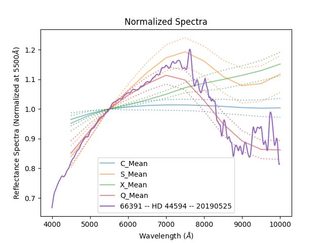
the radar beam width. Astrometric measurements also allow for the detec-
tion and measurement of the Yarkovsky effect on NEOs. The photometric and
spectroscopic data allows us to determine the light curve shape and ampli-
tude, measure rotation periods, determine the taxonomic classification, and
improve the overall characterization of these targets. We are also using a small
amount of the LCO NEO Follow-up Network time to confirm newly detected
NEO candidates produced by the major sky surveys such as ATLAS, Catalina
Sky Survey (CSS) and PanSTARRS (PS1). We will describe the construction of
the NEOexchange NEO follow-up portal and the development and deployment
methodology adopted which allows the software to be packaged and deployed
anywhere, including in off-site cloud services. This allows professionals, ama-
teurs, and citizen scientists to plan, schedule and analyze NEO imaging and
spectroscopy data using the LCO network and acts as a coordination hub for
the NEO follow-up efforts. We illustrate the capabilities of NEOexchange and
the LCO NEO Follow-up Network with examples of first period determinations
for radar-targeted NEOs and its use to plan and execute multi-site photometric
and spectroscopic observations of (66391) 1999 KW4, the subject of the most
recent planetary defence exercise campaign.
Keywords: Asteroids – Near-Earth object – Experimental techniques –
astrometry – photometry

1. Introduction

    Near Earth Objects (NEOs) are our closest neighbors and research into them
is important not only for understanding the Solar System’s origin and evolu-
tion, but also to understand the consequences of, and to protect human society
from, potential impacts. NEOs consist of two subclasses, Near Earth Aster-
oids (NEAs) and a smaller fraction of Near Earth Comets (NECs). NECs are
thought to be extinct comets that originally came from the Kuiper Belt or Oort
Cloud, whereas NEAs originate in collisions between bodies in the main aster-
oid belt and have found their way into near-Earth space via complex dynamical
interactions. Understanding these interactions, the populations of the source re-
gions, and the resulting orbital element distributions requires accurate orbits for
robust samples of the NEO population. Substantial numbers of objects must
be observed in order to properly debias the sample and correctly model the
NEO population. The existing surveys such as the Asteroid Terrestrial-impact
Last Alert System (ATLAS; Tonry et al. 2018), Catalina Sky Survey (CSS), the
PanSTARRS1 (PS1) & PanSTARRS2 (PS2) surveys (Wainscoat et al., 2014)
and NEOWISE (Mainzer et al., 2014) are not normally capable of following-up
their own NEO candidate detections and require additional programs of NEO
follow-up on other telescopes to confirm and characterize the new NEOs.
    LCO has deployed a homogeneous telescope network of ten 1-meter tele-
scopes and ten 0.4-meter telescopes to six locations in the northern and south-
ern hemispheres. These have joined the two existing 2-meter Faulkes telescopes

                                        2
Figure 1: Network map of LCO facilities
(FTN & FTS). The global coverage of this network and the apertures of tele-
scope available make the LCO network ideal for follow-up and characterization
of Solar System objects in general and for Near-Earth Objects (NEOs) in par-
ticular.
We describe the creation, including the testing and software development
philosophy, of the “LCO NEO Follow-up Network” and the central observing
portal, NEOexchange (often abbreviated as ‘NEOx’), in Section 3. We illustrate
the use of the LCO NEO Follow-up Network in Section 4 to perform the science
cases of NEO candidate follow-up and NEO characterization described above.
We summarize some of the results to date and outline plans for future work and
development in Section 5.
2. Overview of the LCO Network
LCO completed the first phase of the deployment (see Figure 1) with the
installation and commissioning of the ten 1-meter telescopes at McDonald Ob-
servatory (Texas), Cerro Tololo (Chile), SAAO (South Africa) and Siding Spring
Observatory (Australia). These 1-meter telescopes join the two existing 2-meter
Faulkes Telescopes which LCO has operated since 2005. The whole telescope
network has been fully operational since 2014 May, and observations are exe-
cuted remotely and robotically. Two additional 1-meter telescopes for the site
in the Canary Islands will be deployed during 2020–2021. Future expansion to
a site at Ali Observatory, Tibet is also planned, but the timescale is uncertain
and dependent on partner funding.
The 2-meter FTN and FTS telescopes originally had identical 100 × 100 field
of view (FOV) Charge Coupled Device (CCD) imager with 18 filters and a low-
3resolution (R ∼ 400, 320 – 1000 nm) FLOYDS spectrograph. The imager on
the FTN telescope on Maui, HI was replaced in 2020 November with a copy of
the MuSCAT2 (Narita et al., 2019) four-channel instrument called MuSCAT3
(Narita et al., 2020). The 1-meter telescopes have a 260 × 260 FOV CCD with
21 filters. Each site also has a single high-resolution (R ∼ 53,000) NRES echelle
spectrograph (Eastman et al., 2014; Siverd et al., 2018) with a fiber feed from
one or more 1-meter telescopes. More details of the telescopes and the network
are given in Brown et al. (2013).
For use in the LCO NEO Follow-up Network for follow-up and characteriza-
tion we primarily make use of the 1-meter network, with some brighter targets
being observed on the 0.4-meter telescopes. Low resolution spectroscopic obser-
vations of NEOs are carried out on the 2-meter FTN and FTS telescopes. With
the deployment of the new MuSCAT3 instrument to FTN, which makes use of
dichroics to provide simultaneous four-color imaging in g 0 r0 i0 zs filters, we have a
powerful tool for simultaneous color and coarse taxonomy determination. This
is particularly true for rapid response characterization of small diameter NEOs
which would be too faint for spectroscopy.
3. Overview of the LCO NEO Follow-up Portal: NEOExchange
We consider NEOexchange to be an example of what are now being called
Target and Observation Management (TOM) systems (Street et al., 2018). The
goal of these systems is to ingest a large number of targets of interest and carry
out selection of a subset according to some merit function. This subset is then
evaluated for observing feasibility and follow-up observations are requested from
available telescopes. The resulting status and any data from these observations
are returned to the TOM system, which records these details. The results of
data reduction on the data are also recorded and this is used as feedback into the
next round of observation planning. NEOexchange is an implementation of such
a TOM system, focusing on Solar System bodies, with a particular emphasis on
NEOs. An outline of the NEOexchange system is shown graphically in Figure 2.
The major sections of the NEOexchange TOM system are the sources of
targets, the database and associated web front-end and interaction tools, the
planning and scheduling functions, and the data reduction processes. Each of
these will be treated in more detail in the following sections.
3.1. Data sources and ingest
The major source of target Solar System bodies is the Minor Planet Center
(MPC), specifically the MPC’s NEO Confirmation Page (NEOCP).1 This web-
page is parsed to extract the NEO candidates from the surveys that are in need
of confirmation. Metadata for each candidate such as the digest2 (Keys et al.,
2019) score (ranging from 0 . . . 100, based on how NEO-like the orbit is), arc
1 https://www.minorplanetcenter.net/iau/NEO/toconfirm_tabular.html
4Figure 2: Schematic overview of the NEOexchange TOM system. Targets for follow-up are
ingested into the NEOx DB (center) from the data source (left side), planned and scheduled
and sent to follow-up telescopes (right). The resulting data flows through the observatory
data reduction pipeline and into the archive. This is retrieved by NEOexchange and processed
through science specific pipelines and the results of these are also stored in the NEOx DB.
5length, discovery and last observed times are extracted. The orbital elements
and observations (in MPC1992 format) are downloaded from the corresponding
links. All of these data are ingested into the NEOexchange database, updating
or creating new records for each of the targets as appropriate.
In addition to the candidates on the NEOCP, we also fetch and parse the
list of cross-identifications of objects that were previously on the NEOCP. This
allows us to learn the fate of the NEO candidates and update our stored state
of the candidates appropriately. This includes when they are designated as a
new object, linked with an existing object (either natural or artificial) by the
MPC, or the candidate is withdrawn or lost for lack of follow-up or failure to
recover it.
Additional sources of targets for characterization efforts (as discussed in more
detail in Section 4.3) are the planetary radar target lists for Goldstone2 and
Arecibo3 . These are supplemented by potential mission destinations from the
Human Space Flight Accessible Targets Study (NHATS) database. The radar
targets are obtained by fetching and parsing webpages, whereas the NHATS
targets are obtained by parsing emails sent to a mailing list. Both of these
methods are somewhat fragile and at risk of missing or misparsing targets if the
webpage or email format changes. This illustrates the need for a lightweight
protocol that can be used by data requestors to signal targets of interest in a
way that is easy and simple to implement as well as parseable and readable by
both machines and humans.
Given a list of characterization targets from any of these methods, we then
make additional queries in the MPC database in order to extract and store
or update the orbital elements of these targets. At present this is also done
by parsing webpages (using the BeautifulSoup4 library), but the MPC has
expressed desires to implement a webservices application programming interface
(API) that provides this information in a more robust manner in the future. We
will implement and switch to this method of obtaining the information once it
becomes available.
Our final source of requests for an increased priority of a particular NEO
candidate is from the JPL SCOUT4 system. This performs analysis of the
short-arc NEO candidates that are on the NEOCP and determines if there is
any risk of a potential impact or close passage to the Earth. Alerts from the
SCOUT system are sent out via email and these can result in the triggering of
follow-up, including potentially disruptive ‘rapid response’ that can interrupt
already running observations on the LCO network.
For the NEO candidates from the NEOCP, tasks are periodically executed
to update the target lists and cross identifications from the MPC. In the case of
the radar and other characterization targets, we update the observations stored
in the NEOexchange database (DB) and perform orbit fitting to update the
2 https://echo.jpl.nasa.gov/asteroids/goldstone_asteroid_schedule.html
3 http://www.naic.edu/
~pradar/
4 https://cneos.jpl.nasa.gov/scout/
6orbital elements to the current epoch. The orbit fitting is performed using the
find orb5 code in a non-interactive mode with the orbit fit to the measurements
for the object exported from the database. These tasks are performed with a
frequency determined by the typical update frequency of the data source. This
is balanced in order to avoid putting undue strain on the remote data source. In
the case of the NEO candidates, updates occur every 30 minutes; for the much
smaller and less dynamic list of characterization targets, the update tasks are
run twice a day.
3.2. Database, web front-end, and user tools
The targets for follow-up and their associated metadata as described in the
previous section, are persisted in a SQL database. This is supplemented by
information on user and proposal details for follow-up resources, follow-up re-
quests, data frames obtained, and the catalog products and source measure-
ments derived from those data frames. An overall database schema is shown in
Figure 3.
We use the Python web framework, Django 6 , to provide a vendor-independent
database abstraction and web front-end. Django provides a means to define
a model of a particular object (such as an asteroid target) and the relevant
concepts and parameters that are associated with that object, and then have
the resulting database table created automatically without the user needing to
worry about the low-level database details. It also provides a means to define
functions on the model that can provide associated calculations such as a sky
position computed from the target model’s orbital elements.
As shown in Figure 3, the database structure is divided into 3 main areas:
• the Body table and related tables which store additional information (the
ColorValues, Designations, PhysicalParameters, PreviousSpectra
and SpectralInfo tables). These tables hold the details about the tar-
gets (such as target type, the data’s origin, orbital elements) and any past
color or taxonomic determinations,
• the SuperBlock and Block tables that record the details of scheduled ob-
servational follow-up, along with the ancillary StaticSource which holds
details about static (sidereal) calibration targets,
• the Frame table, which stores the metadata about our and others’ obser-
vations and associated derived quantities resulting from the observed data
frames and their data processing. These include the CatalogSources ta-
ble (the largest in the DB) which holds the source catalog extracted from
every frame and the SourceMeasurement table which records definite de-
tections and measurements of a particular Body
5 https://www.projectpluto.com/find_orb.htm
6 https://www.djangoproject.com
7Figure 3: Overview of the NEOexchange database schema. Django Model classes become
tables in the database, which are shown as rectangles in the figure with the class/table name
on the top. Primary and foreign keys are shown in bold within the tables and the relationships
between the tables are shown as black lines between the tables.
8In addition to these major tables, there are a small number of ancillary tables to
hold details about the registered users and proposals for the LCO network and
an associated table to link users to proposals, which verifies if they are allowed
to submit observations to the telescopes.
The primary mode of user interaction with NEOexchange is through the web
front-end. This allows users to view prioritized lists of targets, example details
of the targets and the data obtained for them so far. Users can also schedule
additional follow-up observations as well as analyze and report data. Certain
functions, such as submitting observations, require that the user is registered
and authenticated with NEOexchange and has been associated with a proposal
(or proposals) that have time on the LCO network.
In addition to the website, various other command-line tools interact with
the database. These include those that update the target lists described in
the previous section, data download and processing scripts (discussed in Sec-
tion 3.4), and data analysis tools that can build light curves of targets that have
been observed and processed.
3.3. Planning and scheduling
For the purposes of ranking NEO candidates, we compute the following merit
function for each candidate:
tlast 1 1
F OM = e tarc − 1 + e V − 1 + e H − 1
−0.5×(score−100)2
−0.5×(SP D−60.)2
(1)
10 180
+ 0.5 × e +e
where tlast is the time since the object was last seen in decimal days, tarc is
the arc length, also in decimal days, V is the current visual magnitude, score
is the NEOCP digest2 score, H is the absolute magnitude (approx. diameter,
assuming an albedo) and SP D is the South Polar Distance in degrees.
This merit function prioritizes targets that have not been seen in a while,
have a short arc, have a large diameter (small value of H) and are bright,
have a high likely NEO ‘score’, and will go directly overhead of our southern
hemisphere sites (this last weighting factor is because the LCO network has
many more telescopes in the southern hemisphere; see Figure 1). The first
three terms for ‘last seen’/‘arc length’, V magnitude, and absolute magnitude
(H) in the FOM computation are exponential i.e., for brighter, larger, seen less
recently, shorter arc targets, the FOM rises exponentially. The remaining terms
involving the ‘score’ and south polar distance (SPD) are gaussian, where the
expected values are 100 and 60 deg, respectively. The ‘score’ term is weighted
lower (multiplied by 0.5) than the others to avoid it dominating the priority
ranking. The ‘not seen’ and ‘arc length’ parameters are linked together such
that targets with high ‘not seen’ values and low ‘arc length’ values (those that
haven’t been seen in a while and have short arcs) are ranked higher than those
with both values high (those that haven’t been seen in a while and have longer
arcs) or both values low (those that were seen recently and have short arcs).
9In order to calculate the values needed for the merit function above and in
general, the ephemeris calculations make use of the SLALIB library, which has
been wrapped in Python, to handle the position and time calculations. This
library provides the basic functions for the Earth, Moon, and object Cartesian
positions and velocities, precession/nutation matrices and time conversions for
UTC and UT1 to TT and TDB. We have used these routines as the basis for our
code that can calculate the brightness, sky position, motion and angle, altitude,
and moon separation for a particular site as a function of time. The sky motion
is used to set a suitable maximum exposure time that will not produce trailing
beyond the size of the seeing disk. The computed ephemeris is then intersected
with both the calculated darkness times at the site as well as the telescope class-
specific altitude and hour angle limits. The expected brightness of the target is
used to set the length of the requested observation block based on 1 magnitude
bins. The number of exposures of the previously calculated maximum exposure
time that will fit in the block, given the block setup (e.g. slew and settle) and
per-frame overheads is calculated. After review by the user, the observation
request is sent to the LCO observing portal and scheduling system for possible
scheduling on the LCO network.
For spectroscopy observations, the situation is similar but a little more com-
plicated as additional lamp flat and arc calibration observations are also re-
quested, bracketing the main science spectrum. For calculating the expected
signal-to-noise ratio (SNR) on the asteroid target, we make use of a generalized
telescope and instrument model to build an Exposure Time Calculator (ETC).
This makes use of a parameterized taxonomic class to photometric passband
transformation based on Veres et al. (2015) and the mean (S + C) result based
on the findings of Binzel et al. (2015) that S- and C-type asteroids account for
∼ 50 % and ∼ 15 % of all NEOs respectively. We then calculate an effective
capture cross-section based on the unobstructed area of the primary mirror.
This is then reduced by the throughput, expressed as
t = tatm × ttel × tinst × tgrating × tccd (2)
where tatm = 10(−k/2.5)X is the throughput of the atmosphere, with k being
the atmospheric extinction coefficient in the band (in mag/airmass) and X
is the airmass, ttel = 0.85ntel mirr is the telescope throughput with 0.85 being
the typical reflectivity of overcoated aluminium and ntel mirr is the number of
telescope mirrors, tinst is the instrumental throughput (excluding the grating)
which tends to be more uniform with wavelength, tgrating and tccd are the
efficiency of the grating and CCD in the observed band respectively. Slit losses
are calculated based on the width of the slit and the typical FWHM of the
seeing disk.
For the noise sources, we calculate the expected sky background based on
the contributions from airglow (we use the 10.7 cm radio flux data as a proxy
for the progression through the solar cycle which has been shown to correlate
with the airglow intensity e.g. Tapping 2013), zodiacial light (as a function
of ecliptic latitude), the stellar background (as a function of galactic latitude)
10and the Moon. The model for the brightening due to moonlight is based on
Krisciunas and Schaefer (1991). The readout noise per pixel is also included
in the noise sources, though we neglect the dark current as CCD cameras in
spectroscopic instruments are normally operated cold enough that the dark
current is negligible.
We are developing a more sophisticated and generalized ETC which will
make use of an “ETC language” to describe all of the elements and surfaces
(e.g. atmosphere, mirror, lens, grating, CCD etc) and the relationship between
them as encountered by a photon from the top of the atmosphere to the detector.
For each surface, the ETC language will support use of a scalar (e.g. a target V
magnitude), short vector/per-filter values (e.g. extinction per unit airmass as
a function of filter/passband) or a “spectrum” file (e.g. a reflectance spectrum,
measured mirror reflectivity as a function of wavelength). This can be combined
with the selection of the best-matching atmospheric transmission spectrum from
a library of pre-calculated versions (such as the ESO Advanced Sky Model; Noll
et al. 2012) with selection based on the values of precipitable water vapor, ozone
(O3 ) and aerosols determined from remote sensing. This will be described in
more detail in a future publication.
For spectroscopic calibration, nightly flux standards are automatically ob-
served using each FLOYDS instrument. These publicly available flux standards
are used to create an airmass curve and account for nightly perturbations in
atmospheric transmission. Additionally, for Solar System observations, Solar
analogs are required to properly obtain a reflectance spectrum. NEOexchange
is capable of automatically selecting and scheduling a suitable star from a list
of Sun-like options. Stars that are closer on the sky to the target Solar System
object are given preference so that observing conditions might be as similar as
possible between the analog and the primary target. The exposure time of the
analog spectrum is automatically determined based on the brightness of the
analog and the resulting spectra are then stored and uploaded to the NEOex-
change website. Though this process has been fully automated and streamlined,
it should be noted that several fundamental limitations are imposed by the LCO
observing portal and scheduler. The greatest of these limitations is the inability
to create single observations that include multiple targets. Because of this, we
must schedule the target and the analog separately, giving no guarantee that
both will be observed on a given night. As neither observation is complete
without the other, this adds some risk of lost time to Solar System spectro-
scopic observations with LCO. Additionally, due to the constant updating of
the LCO observing schedule, it can be difficult to schedule both target and ana-
log at the same airmass, which is ideal for optimal reduction. We have found,
however, that this latter limitation can be mitigated somewhat by use of the
aforementioned flux standards so long as both observations were made on the
same night.
3.4. Data reduction pipelines
During and after the window of validity of the observing requests, we check
with the LCO observing portal whether the request has been executed on the
11LCO network. If it has, we check with the LCO Science Archive for the pres-
ence of reduced frames. Data taken on the telescopes of the LCO network
are automatically transferred back to the headquarters in Santa Barbara, CA
and pipeline processed. This occurs in near real-time, typically within ∼ 10–
15 minutes of shutter close at the telescope. The pipeline assembles any bias,
dark, or flat field frames that were obtained at the end of the previous night and
start of the current night (and have passed quality control checks) into master
calibration frames. If there are no suitable calibration frames from the current
night, as can sometimes be the case for flat fields in a specific filter, the most
recent master calibration file is retrieved from the calibration library.
The initial data reduction is carried out using the BANZAI pipeline (Mc-
Cully et al., 2018) which performs the standard steps of assembling master
calibration frames from the individual biases, darks, and flat fields. These cal-
ibrations are then applied to the science images to perform bad pixel masking,
bias subtraction, dark current correction, and flat field division. Crosstalk cor-
rection and gain normalization between the individual quadrants and amplifiers
of the Sinistro cameras’ Fairchild CCDs are also performed. An astrometric so-
lution is performed using the astrometry.net software (Lang et al., 2010) which
makes use of the 2MASS catalog (Skrutskie et al., 2006) as input. A catalog of
sources detected in the frame (having a certain minimum number of pixels more
than 10σ above the fitted sky background) is also produced using SExtractor
(Bertin and Arnouts, 1996). Finally the reduced frames, source catalog, and as-
sociated master calibration frames are uploaded to the LCO Science Archive7
for distribution to end-users. These data products are then retrieved by NEOex-
change for further astrometric and photometric analysis.
Although the BANZAI pipeline does a good job at removing the instrumen-
tal signature from the data and providing a “first pass” astrometric solution,
we cannot make use of this pipeline-produced astrometric solution and source
catalog as-is. This is because the camera distortions, although small, are too
large for our astrometry goals to be met with a simple linear fit. In addition,
because many of our NEO targets are very faint, they will not be included
in the relatively shallow pipeline-produced source catalog. To solve both of
these problems, we instead re-determine a new astrometric solution, incorpo-
rating spatially-varying distortion polynomials. This astrometric solution ini-
tially used the PPMXL catalog (Roeser et al., 2010), progressed to using the
Gaia-DR1 catalog (Gaia Collaboration et al., 2016) and now makes use of the
Gaia-DR2 catalog (Gaia Collaboration et al., 2018) to derive the astrometric
solution and a per-frame photometric zeropoint using the SCAMP software8 .
The zeropoint is determined by cross-matching the detected CCD sources
with sources in the Gaia-DR2 catalog by position and then iterating, with out-
lier rejection, to determine the difference in mean magnitude between the in-
strumental CCD magnitudes and the Gaia catalog G magnitudes. This ig-
7 https://archive.lco.global/
8 https://www.astromatic.net/
12nores mismatches between the broad Gaia G passband and the equally broad
PanSTARRS-w, which comprise over 85% of our frames, and does not take
into account the source color (almost always unknown) or stellar color. The
color correction for reference star colors was not possible when this part of the
pipeline was originally written with the absence of accurate colors in either the
PPMXL or Gaia DR1 catalogs. Given the large field of view of the LCO tele-
scopes and the corresponding large number (hundreds) of potential reference
stars in a typical field, the outlier rejection procedure for the zeropoint is robust
against including stars with large discrepancies in color and magnitude. With
the availability of GBP and GRP magnitudes in Gaia DR2, and the prospect of
spectral types for large numbers of reference stars from low resolution spectra
in Gaia DR3, there is the potential to revisit this in the future versions of the
pipeline with an improved treatment.
The result of the fitting process and a record of the resulting processed frame
data product is stored in the database. After checking that the results of the fits
are satisfactory, we perform a source extraction again using the SExtractor
(Bertin and Arnouts, 1996) software but to a lower threshold than in BANZAI
(3.0 vs 10.0 σ above the sky background) to include many more faint sources.
The resulting source catalog contents are ingested into the database (forming
the largest fraction of the database size).
This additional processing allows us to extract light curves for any object in
the database through either user tools or via the web frontend (see Figure 2).
The source catalogs can also be exported to specialized moving object detection
software written by the Catalina Sky Survey team (Shelly, 2016). The results
of any detections are also ingested into the database and can be overlaid in a
“Candidate Analyzer” in the web frontend. This allows the user to blink through
the acquired frames for that candidate object and the moving object detections
are overlaid, along with details about the position (both on the CCD and on-
sky), magnitude, and the rate and direction of motion, allowing comparison with
the predicted motion to assist confirmation of a NEOCP candidate’s recovery.
The user can then reject or confirm the identification which will then show a
summary of the observation in the MPC1992 80 column format which can then
be sent to the MPC. Moving object detections of real but unknown objects can
also be confirmed, in which case a new local candidate object is created in the
database.
As discussed above, we make use of the Gaia-DR1 (Gaia Collaboration et al.,
2016) and Gaia-DR2 (Gaia Collaboration et al., 2018) catalogs to perform the
astrometric reduction. Gaia-DR1 greatly improved the quality of astrometry
obtained by substantially reducing the systematic error contribution by vastly
reducing the catalog zonal errors (Spoto et al., 2017). The overall astrometric
uncertainty is a combination of centroiding error (which is unaffected by the
choice of reference catalog), systematics from the reference catalog and other
normally smaller second-order effects such as stellar proper motion and differ-
ential chromatic refraction.
Switching from PPMXL (Roeser et al., 2010), which we used prior to the
availiability of the Gaia catalogs, to Gaia-DR1/2 has reduced the systematic
13catalog error from ∼ 300 mas to ∼ 30 mas and the overall uncertainty (∼ 0.0800 –
0.2100 ) is now dominated by the centroiding error. With the release of DR2 in
April 2018 and the availability of good reference star colors, as well as the release
of parallaxes and proper motions in later data releases, it would be possible to
take other more subtle effects into account in the astrometric reduction.
These effects include the differential chromatic refraction (DCR), space mo-
tions of the reference stars, and unmodelled optical distortions. DCR is caused
by differences in the spectral energy distribution of the Solar System targets and
reference stars being refracted differently in the atmosphere, which in terms de-
pends on the variation of temperature, pressure and water vapor (Stone, 1996)
both from site to site and with time. The amount of DCR also depends on the
filters used and the optical path length through the atmosphere, which depends
on the (changing) zenith distance and hour angle of the target. Historically, the
lack of even accurate colors for the majority of reference stars, has made correc-
tion of DCR difficult without obtaining large amounts of additional multi-color
calibrated photometry. Similarly correcting for the proper motions, and less
commonly for the parallax, of the reference stars has been difficult due to lack
of accurate available data for the fainter (V ∼ 12–18) stars mostly commonly
used as reference stars for ∼ 0.5–2 m telescopes. Finally, mapping optical dis-
tortions that are not modelled by our use of third order distortion polynomials,
also requires very accurate reference positions in crowded fields, such as star
clusters. With colors, accurate positions and space motions, coming in Gaia
DR3 and subsequent releases, these smaller contributions to the astrometric er-
ror could be modelled and removed. A more detailed modelling and analysis
effort considering the typical targets and observing circumstances of the LCO
NEO Follow-up Network would be needed to assess the relative contributions
of the various sources of astrometric error.
3.4.1. Spectroscopy Reduction
The FLOYDS Spectroscopy Pipeline is automatically run on all FLOYDS
data obtained by the LCO network in a manner similar to the BANZAI pipeline
described above. The pipeline converts the raw, folded, multi-order fits frames
into a 1-dimensional extracted trace of the entire merged spectrum. During
this processing, lamp flats are used to minimize fringing in the red branch, then
stored flux calibration frames and telluric lines are used for atmospheric cor-
rection. The final trace, as well as all intermediate data products, are wrapped
in a tarball along with the guider images and made available to users via the
LCO archive. A full description of the data processing, wavelength calibra-
tion, and extraction is given on the LCO website9 . The data resulting from
this automated pipeline is typically of sufficient quality to determine a rough
spectral slope for the target and serves as a good first look. However, when
higher quality reduction is needed, a manual version of the pipeline can be run
that uses lines from an arc lamp observed before and after the object frames
9 https://lco.global/documentation/data/floyds-pipeline/
14to perform wavelength calibration, as well as more recent flux standards that
can improve atmospheric correction. NEOexchange retrieves these data from
the LCO archive and automatically creates a reflectance spectrum with the
most proximate Solar Analog spectrum observed with the same telescope as the
object of interest.
3.5. Development and Deployment Methodologies
One of the priorities for creating TOM (Target and Observation Manage-
ment) systems like NEOexchange is to allow them to be developed, adapted,
and deployed by different groups for their own particular science interests and
follow-up assets. Furthermore, scientific reproducibility is enhanced by having
the full chain of software that was used to produce a scientific result available,
along with the platforms the software operates on, which can be replicated by
third parties via virtual machines (Morris et al., 2017).
Mindful of the above, we have adopted the following philosophies:
• the use of Python as the programming language,
• the use of version control (git and github.com) to manage revisions to the
software,
• the adoption of Test-Driven Development (TDD) methodologies to de-
velop and maintain the software,
• the use of container technology to package and deploy the running soft-
ware,
The NEOexchange platform is written in Python which has had a high take
up for astronomy software and allows access to a large variety of astronomy-
specific packages such as astropy (Astropy Collaboration et al., 2013) and
astroquery (Ginsburg et al., 2019). This is the most flexible choice at present
for open access astronomy software.
Although the use of Test-Driven Development (TDD) in scientific software
is currently small (Nanthaamornphong and Carver, 2017), it can provide many
benefits. The use of unit tests for the individual low-level functions and func-
tional tests for the overall website operation helps in building more reliable and
maintainable software over the long term. The combination of tests, along with
the use of packaging and deployment technologies (described later), improves
the reproducibility of scientific results by allowing others to reproduce them on
a wide variety of platforms. Given the use of the Python programming language
for NEOexchange, we decided to adopt pytest and Selenium10 for developing
and running the unit and functional tests respectively. This builds on our pre-
vious efforts (e.g. Lister et al. 2016) but uses more modern web development
and deployment frameworks such as Django and Docker to make a redeployable
10 https://www.selenium.dev/documentation/en/webdriver/
15web service that can support many users and multiple projects that are using
the LCO Network.
To allow the NEOx software to run in many more places and to decouple
the code deployment from the underlying hardware and operating system, we
make use of the Docker11 container platform to package and run the software.
Docker has quickly emerged as the technology of choice for software contain-
ers. Docker is an operating system level virtualization environment that uses
software containers to provide isolation between applications (compared to vir-
tual machines (VMs) which virtualize at the hardware level and require a guest
operating system per VM). Through the use of a standardized file format (the
Dockerfile) for describing and managing the setup of the containers, we can
separate the sub-components of NEOexchange (the database, web frontend, and
tasks backend) into standardized containers for each component.
This ability to be able to completely describe a software deployment envi-
ronment with Docker has the potential to improve the reproducibility and the
sharing of data analysis methods and techniques for the science and research
community. This can allow other researchers the ability to reproduce and build
on the original work (e.g. Boettiger 2015) or to develop and distribute con-
tainerized versions of tools (e.g. Nagler et al. 2015) which can otherwise be
hard to install and setup.
It is often the case that the research team developing the software does not
have (or desire) direct control and management over the software environment
where their software will be deployed. The deployment platform may be con-
figured with different versions of the operating system, Python libraries, and
modules than those that are required by their software, and yet are necessary
for the stability and long-term support of other applications. This can present
problems when attempting to update the version of these infrastructure compo-
nents, as it is normally very difficult to isolate the different system components
from each other, requiring all components to be updated at the same time.
With Docker, each application can be wrapped in a container configured
with the specific version of operating system, Python interpreter, and Python
packages and modules it needs to function properly. The common interface with
the system is set at the container level, not at the operating system, program-
ming language, or application server level. In this container-based approach to
deploying a service like NEOexchange, the development process includes a con-
tainer specifically designed for the service, with only the dependencies needed by
the service. The same container that is used during the development and testing
of the NEOexchange software on the developer’s local machine can be deployed
on a local computer cluster or in a private part of a cloud service, and even
becomes part of the final project deliverable. The final product is shipped and
deployed as the container, with all of its dependencies already installed, rather
than as an individual software component which requires a set of libraries and
components that need to be installed along with it. This not only simplifies the
11 https://www.docker.com
16deployment of the final product, it also makes it more reproducible.
For NEOexchange, we use Docker to build two sub-containers, one for fetch-
ing and compiling the find orb12 orbit fitting code (which needs more modern
compilers than our base CentOS13 7 OS image possesses) and one for setting up
the system and Python dependencies. The results are then incorporated into
a third container which includes the necessary system tools (primarily SEx-
tractor, scamp, and the CSS moving object code), the main NEOexchange
application code, and finally the crontab entries used for the object and data
downloads (as described in Section 3.1 and Section 3.4) and other maintenance
tasks. The containers can be built and rebuilt using the Docker command-line
tools and are also rebuilt automatically by the LCO-wide Jenkins14 automated
build servers whenever commits are made to the NEOexchange github reposi-
tory.
For deployment we make use of Amazon Elastic Kubernetes Service (EKS)
to deploy our Docker containers to the Amazon Cloud and allow users to access
the system. Kubernetes15 is a container orchestration system for automating
deployment and management of containerized applications. EKS makes use
of Amazon’s Elastic Compute Cloud (EC2) to provide the virtual servers for
running the NEOexchange application and the S3 storage system to store the
files needed. We use Kubernetes to deploy several containers that setup and
then run the NEOexchange application. Two initialization containers are run at
startup; one collects all of the static content (HTML, CSS, images, JavaScript)
needed by the Django framework and webserver that runs the NEOexchange
application and the other is used to download the DE430 JPL ephemeris file
(Folkner et al., 2014) to the shared S3 storage for use by find orb during orbit
fitting. Following the completed execution of these initialization containers, we
deploy three other containers for the main NEOexchange application. These
are the nginx webserver, the backend NEOexchange application itself, and the
container for running the background and update tasks through the crontab.
The Kubernetes system and the Amazon EKS handles constructing the needed
services to direct web traffic from the internet to the NEOexchange application
and its webserver. It also handles redeploying the NEOexchange containers
should the application or one of the underlying virtual servers go down, or if
an upgrade to a new version of our application is deployed. In the latter case,
the new version is brought up in parallel and confirmed to be working before
routing traffic over from the old version, at which point the older deployed
version is removed. Kubernetes also allows us to run a developmental version of
the NEOexchange code in parallel, using a separated parallel database, without
disturbing the production system. This allows us to build additional confidence
that the system and any new features are working correctly, beyond the checks
12 https://www.projectpluto.com/find_orb.htm
13 https://www.centos.org
14 https://jenkins.io
15 https://kubernetes.io
17of our unit and functional tests, before making the new version live.
The use of a common, widely adopted programming language and web frame-
work, coupled with modern software development methodologies, particularly
Test Driven Development, has enabled us to develop and add many new fea-
tures to the NEOexchange codebase while ensuring that the code continues to
work as expected. The adoption of containerizing technologies to package the
software and all needed dependencies has also, after an initially steep learn-
ing curve, been greatly beneficial in that it has served to insulate the code
and ourselves from many of the demands and trials of system administration.
The more recent move to a more virtualized deployment strategy using cloud-
based services, has similarly produced great medium and long-term benefits by
allowing NEOexchange to be kept continuously running during seamless and
safe upgrades alongside parallel deployments for testing of new versions without
impact to the production system.
4. Use of the LCO Network for NEO follow-up and characterization
4.1. Follow-up for NEO Surveys (PS1 & 2, CSS, NEOWISE & others)
One of the original motivations for building the NEOexchange system (and
its predecessor) was the large number of NEO candidates produced by the NEO
sky surveys (thousands/year) requiring follow-up confirmation through astrom-
etry and photometry. As described in Sections 3.1 and 3.3, the NEOexchange
system retrieves new NEO candidates from the MPC, computes ephemerides,
and can plan observations and automatically schedule them for follow-up on the
robotic telescopes of the LCO network.
The NEOexchange homepage shows the candidates in need of follow-up,
ranked according to the FOM equation (Equation (1) and Section 3.3) along
with recently confirmed NEOs. Individual candidates can be scheduled from
here by following their associated links. There is also a command line user tool
which can look at the current state of the candidate follow-up needs by query-
ing the database and the state of the telescope network and then distributing
candidates to available telescopes at a given time (planning for a future time is
supported). By default, this tool retrieves all of the NEOCP candidates that
were ingested into the database within the last 5 days. In addition to older ob-
jects, we also filter out those that have not already been followed up and those
that haven’t gone more than 2.5 days without being observed. These cuts are
necessary as the short ∼ 30 minute discovery arc of typical NEOCP candidates
means that their positional uncertainty can grow to many times our field of view
after this time. All of these cuts can be customized by the user using command
line options.
For each of the selected candidates, we compute the ephemeris and they are
then filtered as follows:
• V magnitude in the range 19 ≤ V ≤ 22,
• on-sky motion ≤ 500 /min,
18• Moon-object separation ≥ 30◦ ,
• not already scheduled to be observed by NEOexchange
Filtered objects are then split into four lists : first by declination (Objects with
Dec. +5◦ go
into the northern hemisphere list), and then into a “telescope class” list with
V ≤ 20.5 objects going to the 0.4 m telescopes and fainter to the 1 m telescopes.
This allows the targets to be directed to the telescope class that is optimal for
their brightness.
Once the NEOCP candidates have been filtered and sorted, the currently
dark subset of the LCO network is checked for an operational status through
an LCO-provided API. The targets are then scheduled on the appropriate site
and telescope class. We operate by sending NEOCP candidates to a specific
site, rather than using the more common mode of submitting to the whole LCO
network with a longer possible observing window, because we are interested in
getting new measurements as soon as possible. By submitting to each site in
turn as the Earth rotates we can optimize the time to a result and subsequent
resubmits of the observation request will use the most current knowledge of the
candidate’s orbit at that time. We continue submitting requests for observa-
tions until either we get data or the object is confirmed by other observers and
designated by the MPC.
After observation of the requested targets has occurred and the data has
been processed as described in Section 3.4, candidates that have been auto-
matically detected by the moving object code are presented in NEOexchange.
After checking the validity of the observations by including them in a combined
fit with the existing measurements (downloaded from NEOexchange) using the
find orb orbit fitter, the measurements are sent to the MPC. For targets which
are not automatically identified or which are moving too fast to be identified
in the individual frames and which require stacking on the object’s motion, the
data is downloaded and analyzed on a local workstation. Manually detected
objects have their measurements checked for validity and then are reported to
the MPC in the same way as described above.
4.2. Rapid response to close-passing objects
The combination of a large number of telescopes distributed around the
world, coupled with the ability of the LCO scheduler and the site software
to re-plan, schedule and start execution of a new observing request within
∼ 15 minutes, allows the LCO network to respond rapidly to new targets of
opportunity. These objects are primarily those NEO candidates that are deter-
mined to have a possibility of impact by the JPL SCOUT early alert system.
Since the particular candidate will already be in the NEOexchange system from
an earlier ingest of candidates (see Section 3.1), all that is necessary is to trigger
a disruptive rapid-response request. This involves setting a particular value of
the observing mode in the observing request which tells the LCO system that
this request is of high enough priority that it can potentially disrupt and cancel
19an already running request at the telescope. This can be done through either
the web frontend when scheduling an object or by adding a flag to the command
line tool that was described in Section 4.1.
These rapid-response observations are considered first by the LCO scheduler
in a separate scheduling run and sent out to the sites, before the rest of the
observing requests are scheduled, which reduces the latency. Once executed at
the telescope, the resulting data is treated in the same way as that from other
targets.
As briefly discussed for NHATS and SCOUT targets in Section 3.1, there is
a need for a better machine-readable format for requesting transient follow-up
generally. Although the original SCOUT email alerts (which were machine gen-
erated and also semi-structured and machine readable to some extent) have now
been supplemented by an API endpoint, the subsequent discussion about the na-
ture of the object and validity of the alert and recommendations for continuing
or halting follow-up are all conducted through free-form email conversations.
This is also the situation in a number of other of time-domain and transient
astronomy fields and illustrates the need to take the “next step” to allow better,
faster, and more automated responses to, and prioritization of, new transients.
This extends the potential for automation and faster response further down the
chain from the producers of alerts and the broker/triage stage to follow-up and
characterization resources, as has already been done by many surveys e.g. ZTF
(Patterson et al., 2019).
4.3. Follow-up of radar-targeted NEOs and Potential Mission Destinations
Radar observations are a very powerful tool that are used to spatially resolve
NEO targets, determine binary fraction and improve orbits, the last of which
helps us to avoid loosing the target and improves impact risk assessment (e.g.
Ostro et al. 2007). The LCO NEO Follow-up Network allows rapid response
astrometry that makes pointing and imaging by radar assets (such as Gold-
stone and Arecibo) possible for targets that have only recently been discovered.
Potential mission destinations such as NEO Human Space Flight Accessible
Targets Study (NHATS) targets are often small in size with a limited visibility
window of days to a few weeks. The LCO NEO Follow-up Network can quickly
respond for characterization efforts for these objects. The network can also
obtain colors and photometric light curves which allows the determination of
rotation rates, pole directions, spectral classes, and shapes as well as perform
robotic spectroscopy to determine taxonomic classes. The majority of our time
allocation for the project is now spent on characterization efforts for these types
of targets.
In addition to the ingest of the characterization targets discussed in Sec-
tion 3.1, we also ingest any known physical parameters such as a light curve
period and amplitude, pole orientation, and taxonomic class if known. This is
performed via a query and parsing of the JPL Small Body Database and storage
of the results. In the absence of a period, we perform an initial observation block
of 1 hr in the PanSTARRS-w filter for maximum throughput, with the expo-
sure time automatically calculated based on the object’s speed as described in
20Figure 4: Example NEO light curves obtained with LCO NEO Follow-up Network: Light
curve from the 0.4-m telescope in Tenerife (MPC site/telescope code Z17) of NEO (3122)
Florence (left) which was observed with the Goldstone radar in 2017 August–September and
was discovered to be a rare triple system and a light curve of NEO 2015 EG from the LCO 1-m
in Chile (MPC site/telescope code W86) on 2019 March 6 (right) which was also observed that
month by the Arecibo planetary radar. The right figure shows an example of the automatically
produced plot products, with the light curve plotted on top with the pipeline-determined per-
frame zeropoint underneath.
Section 3.3. Following the results of these initial observations, further follow-up
falls into one of three categories:
1. The block covered at least ∼ 1.5× the period: period is determined and
announced to community. Move onto taxonomic spectroscopy (for V .
17) or colors (for V . 20.5).
2. Initial block indicates period in the 1 . . . 4 hr range: Longer block scheduled
to capture the full period.
3. No indication of a period: Cadence scheduled covering 2–3 days with
observations every 20–60 minutes.
Examples of the follow-up photometry for period determination that were ob-
tained for two radar-targeted NEOs are shown in Figure 4. (3122) Florence is a
large ∼4.2 km (using the MPC HV = 14.1 value and the NEOWISE albedo of
0.231; Mainzer et al. 2011) Earth-approaching Amor NEO which made a close
(∼0.047 au) approach to the Earth in 2017 September; this was the closest ap-
proach until the 2057 apparition, making it an important opportunity to study
this potentially very damaging large NEO. It was also the target of a citizen
science Asteroid Tracker campaign for that year (see Section 4.4).
Observations were carried out with the southern 1-meter telescopes and
northern 0.4-meter telescopes of the LCO network prior to and following close
approach respectively. One of the light curves from one of the northern 0.4-
meter telescopes in Tenerife (which has a MPC site/telescope code of Z17) is
shown in Figure 4.3. These data confirmed the 2.36 hr period found in the 1996–
1997 apparition by Pravec et al. (1998). (3122) was subsequently shown to be
a triple system with 2 small companions in radar images.
212015 EG was discovered by Catalina Sky Survey’s Mount Lemmon Station
in 2015 March and its Earth-crossing short period (P ∼293 day) and eccentric
(e∼0.36) Aten orbit means it makes frequent close approaches to both Earth and
Venus. It was targeted by the Arecibo planetary radar on the next return in 2019
March, five orbital periods later. A 1.7 hour observation block two days after
closest approach with the LCO 1-meter at Cerro Tololo (MPC site/telescope
code W86) showed a complex light curve with two unequal maxima and minima
(Figure 4.3). The existence of distinct maxima and minima in the light curve
suggests an elongated shape but the fact that the two maxima and two minima
are themselves unequal, shows that the situation is more complicated. This
would need a more thorough light curve inversion, ideally incorporating the
radar data in a combined solution. We determine a period of ∼0.717 hours based
on the two maxima, in contrast to the previous determination of 1.29 hours
of Thirouin et al. (2016), which was an estimate based on incomplete phase
coverage. The radar ranging also secured a provisional weak detection of the
Yarkovsky acceleration (see next section) on this object, making the Yarkovsky
acceleration a more secure 2.4σ detection.
4.3.1. Yarkovsky measurements
The semi-major axis drift some asteroids undergo due to the non-gravitational
Yarkovsky effect, caused by the unequal absorption and re-radiation of thermal
energy on a rotating asteroid, can have a large influence on determining impact
probabilities for asteroids that pass close to the Earth (Giorgini et al. 2002,
2008; Farnocchia et al. 2013; Farnocchia et al. 2014; Chesley et al. 2014; Spoto
et al. 2014; Vokrouhlický et al. 2015). Even a small drift in semimajor axis can
make the difference between a near-miss and an impact for close-passing aster-
oids when calculating long-term impact probabilities, especially when planetary
close encounters perturb the orbit.
The various command-line tools available through NEOexchange (described
in Section 3.2) were used to calculate the observability, brightness, and rate of
motion of 36 asteroids determined to yield a high likelihood of a detection of
the non-gravitational Yarkovsky effect (Greenstreet et al., 2019). The targets
were ingested into the NEOexchange database, which allowed for ephemeris
calculation, planning, and scheduling of observations on the LCO network.
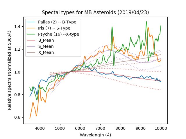
4.3.2. Robotic spectroscopic characterization
Through the robotic FLOYDS spectrographs on the two 2-m telescopes
on Maui, HI and Siding Spring, Australia (see Figure 1), we can perform
rapid-response low resolution spectroscopy of NEOs and other asteroids. Af-
ter scheduling of spectroscopic observations (described in Section 3.3) and data
reduction (described in Section 3.4), the data products for the target and the so-
lar analog are extracted and made available through the NEOexchange website
from the requested observation block. This also allows display and download of
the acquisition and guide movies made from the autoguider frames taken during
the observations.
22You can also read