Nonlinear dynamic soil structure interaction in adjacent basement - IOPscience
←
→
Page content transcription
If your browser does not render page correctly, please read the page content below

IOP Conference Series: Materials Science and Engineering

PAPER • OPEN ACCESS

Nonlinear dynamic soil structure interaction in adjacent basement
To cite this article: Yetty Saragi et al 2020 IOP Conf. Ser.: Mater. Sci. Eng. 725 012031

View the article online for updates and enhancements.

                                This content was downloaded from IP address 46.4.80.155 on 22/11/2020 at 15:34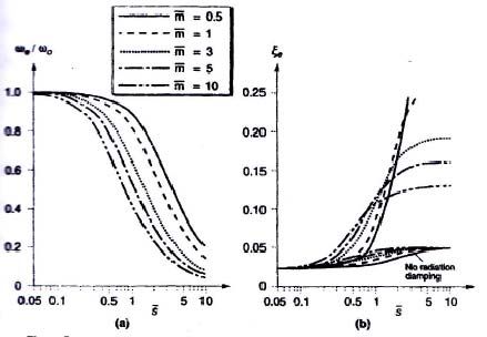
3rd NICTE                                                                                  IOP Publishing
IOP Conf. Series: Materials Science and Engineering 725 (2020) 012031 doi:10.1088/1757-899X/725/1/012031

   Nonlinear dynamic soil structure interaction in adjacent basement
                    Yetty Saragi1*, Masyhur Irsyam2, Roesyanto3, Hendriyawan2
                    1
                      Postgraduate Student of Departement Civil Engineering, University of North
                    Sumatera (USU)
                    2
                      Study Program of Civil Engineering, Institute of Technolgy Bandung (ITB)
                    3
                      Departement Civil Engineering, University of North Sumatera (USU)
                    *yettyririssaragi@yahoo.com

                    Abstract. This research was conducted to analyze the lateral dynamic pressure
                    distribution on the basement walls and amplification of earthquake motion on the
                    surface using the finite element method Midas GTS-NX. Dynamic soil-structure
                    interaction analysis was carried out by using a sensitivity program to influence
                    soil conditions, earthquake acceleration in bedrock, basement depth, bedrock
                    depth and stiffness of the basement structure with a distance between basements
                    of 15,0 m. From this study, the lateral pressure distribution of the dynamic soil
                    reaches the maximum at the base of the basement with an increase in pressure that
                    is almost linear in soft and nonlinear soil conditions in medium and hard soil
                    conditions. The greatest increase in gradient occurs at a depth of four per five
                    basement walls measured from the surface to the bottom of the basement. The
                    analysis shows that the dynamic lateral pressure distribution has a maximum
                    value at the top end of the basement and tends to shrink to the bottom of the
                    basement.

        1. Introduction
        High-level building structure in general can be divided into two main parts, namely the
   structure of the building which is above the ground surface and the structure of the building
   that is below the surface of the land. The structure of the building below the ground surface
   can be in the form of a basement called a basement. The function of the basement is to carry
   the weight of the upper structure into the soil and to resist lateral loads around the basement
   wall. One aspect of geotechnics that is often a problem in basement wall planning is the
   determination of lateral ground pressure in the basement wall due to earthquake which must
   be held by the basement wall. Therefore, it is necessary to analyze the interaction of the soil
   with the basement structure walls on the dynamic response. Research on interactions that
   occur between soil and structure has also been carried out, in order to obtain influence due to
   seismic loads (Sherif and Famg, 1984; Ishibasi and Fang, 1987; Wu and Finn, 1996;
   Hendriyawan and Meddi, 1996; Putu Sumiharta, 2002; I Nengah Sukertha, 2008; Imanuel
   Mangape, 2009). Further studies and analyzes are still needed to obtain more detailed
   dynamic response behavior of the soil-structure of the basement wall.
        In this research, an analysis of the effect of local soil conditions on the interaction of soil
   dynamic responses to the basement wall structure is in the form of non-linear soil behavior in
   the form of a comparative study of the response of equivalent linear and nonlinear soil models
   to the basement wall structure which is also influenced by bedrock depth and acceleration
   surface earthquake waves.

              Content from this work may be used under the terms of the Creative Commons Attribution 3.0 licence. Any further distribution
              of this work must maintain attribution to the author(s) and the title of the work, journal citation and DOI.
Published under licence by IOP Publishing Ltd                          1
3rd NICTE IOP Publishing
IOP Conf. Series: Materials Science and Engineering 725 (2020) 012031 doi:10.1088/1757-899X/725/1/012031
2. Methodology
2.1. Soil structur interaction
Building construction based on its location to the ground surface can be divided into 2
(two) parts, namely the upper structure (upper structure) and the lower structure (sub
structure). Both parts of this building have several differences in the method of analysis for
design purposes. The difference is caused by differences in environmental conditions around
the two parts of the construction building. For the upper structure, the state of the land does
not directly influence the process of analysis and design. Meddi R. and Hendriyawan (1996)
in their research results stated that for lower structures or embedded structures, the state of the
soil plays an important role in the design of the external forces at work so that interactions
between the soil and embedded structures need to be taken into account.
Interactions that occur can be in the form of the influence of earthquake loads on the
dynamic response of the underground structure, or it can be the other way around, namely the
influence of underground structures on the behavior of earthquake wave propagation from
bedrock to surface. The type of material on the bedrock with characteristics of mass and
stiffness will determine how much the earthquake load of the bedrock will change when the
earthquake waves reach the surface. Analysis of lateral ground pressure in this study will use
the help of the finite element program Midas GTS. Soil-structure interaction can be analyzed
by 2 (two) methods, namely the direct method and the stepwise method (Kramer, Steven L.,
1996). The system response is formulated as follows:
M u K u M u ff (t )
(1)
where u ff (t ) is the acceleration of the free field at the nodal point boundary
Deformation in kinematic interactions can be calculated assuming that the foundation has
rigidity but does not have mass. Kramer, 1996 states the equation of motion to represent this
state, namely:
M soil u K I K u K I M soil u b (t )
(2)
Analysis of kinematic interactions results in the movement (relative to bedrock) of a
foundation-structure system that has no mass due to kinematic interactions. This movement is
combined with the movement of bedrock to obtain the total kinematic movement of the
foundation-structure system and produce equation (3)
M u K u M u b (t )
(3)
Kartawijaya, Paulus (2007) mentioned that the soil-structure interaction causes an
interaction force in the soil-structure interface that causes random waves and spreads to
infinity, which is called radial damping. Soil materials provide attenuation called material
attenuation.
The effect of soil-structure interaction on natural frequencies, damping ratios and
displacement characteristics of the equivalent SDOF system can be shown in Figure 1 below.
Figure 1 (a) shows that the natural frequency of an equivalent SDOF system is under a fixed-
base system in addition to the stiffness ratio. The effect of soil-structure interaction on natural
23rd NICTE IOP Publishing
IOP Conf. Series: Materials Science and Engineering 725 (2020) 012031 doi:10.1088/1757-899X/725/1/012031
frequency is slightly below the stiffness ratio, i.e when the soil stiffness is relatively large
relative to the stiffness of the structure. For a fixed-base condition, the natural frequency of
the equivalent system is the same as the natural frequency in the fixed-base condition.
Figure 1. Effect of stiffness ratio and mass ratio on (a) natural frequency, (b) damping ratio of
the soil-structure system ( h 1, v 0.33, 0.025, g 0.05) (after Wolf, 1985)
Figure 1 (b) shows the effect of the soil-structure interaction on the damping ratio for the
equivalent SDOF system. For fixed-base conditions, the damping ratio of the equivalent
system is the same as the structural damping ratio, but as long as the stiffness ratio increases,
the effect of soil attenuation will be more visible. At high stiffness ratios, structural damping
is only a small part of the total damping in the system.
2.2 Dynamic Lateral Earth Pressure Analysis
This method is a modification method from the method that had been developed by
Coulomb (1776). Mononobe and Okabe added additional vertical and horizontal forces due to
the earthquake to the previous calculation. The basic equation of the Mononobe-Okabe
method is the equilibrium of forces acting on a wedge (wedge) as below:
1
PAE = H 2 (1 k v )K AE (4)
2
with,
Cos 2 ( )
KAE = 2
Sin ( ) Sin ( i)
Cos Cos 2 Cos ( )1
Cos ( ) Cos (i )
and,
kh
= tan 1
1 k v
where ,
33rd NICTE IOP Publishing
IOP Conf. Series: Materials Science and Engineering 725 (2020) 012031 doi:10.1088/1757-899X/725/1/012031
= shear angle in the ground
= sliding angle of the wall
i = inclination of land surface is behind the wall
= back wall's slope to the vertical plane
W = weight of the collapse
PAE = active pressure
R = resultant forces along the plane of collapse
khW = internal horizontal force due to weight alone
kvW = vertical internal forces due to own weight
= soil density
KAE = coefficient of active earth pressure with earthquake effects
Figure 2 shows the experimental results of Sherif and Fang (1984) in the form of dynamic
active earth pressure distribution as a function of acceleration in a rigid wall that rotates at the
top.It appears that at the bottom of the wall the value of the soil pressure is almost zero. While
the peak is not zero and the amount increases according to the acceleration increase. The
results of this experiment are in accordance with the predictions of Scott (1973), Matsuo and
Ohara (1960) and Wood (1973).
Maximum Dynamic Earth Pressure (AE )max , (kN/m2 )
2 4 6 8 10 12
0
kh= 0.0 Wall mode : ROTATION ABOUT THE TOP
Static Test Soil Sample : Dense Ottawa Sand
(Experimental) Exp. Result :
20 M-O Solution :
kh= 0.40
Depth, z (cm)
(Experimental)
40
kh= 0.26 kh = 0.52 (Experimental)
60 (Experimental) kh
=0
kh .40 kh =
= (M 0 .5 2
0.2 -O (M
6 ) ono
80
kh
(M n obe
-O
=0
) -Ok
abe
.0
's Sol
(M
utio
-O
n)
)
Figure 2 . Distribution of active active ground pressure rotating at the top as a function of
horizontal acceleration (Sherif & Fang, 1984)
The results of these experiments can be concluded:
a. The dynamic active pressure distribution behind the rotating wall at the top is non-
linear and the magnitude of this pressure reaches zero at the bottom of the wall. This
active pressure increases at a distance of one third from the top of the wall.
b. The dynamic active pressure at the surface is not zero and the pressure at this surface
increases with increasing acceleration.
c. The total dynamic active pressure capture point is 0.55H from the bottom of the wall
and depends on the acceleration rate.
43rd NICTE IOP Publishing
IOP Conf. Series: Materials Science and Engineering 725 (2020) 012031 doi:10.1088/1757-899X/725/1/012031
3. Result and discussion
The earthquake source zone used in this study is a subduction zone, which is a zone of
earthquake events that occur near the boundary between the oceanic plates that pierce under
the continental plate. The subduction zone referred to in this study is the megathrust zone,
which is a sub-earthquake subduction from the surface to a depth of 50 km. The classification
of local soil is one of the important stages, because different soil classifications will provide
different soil responses in propagating waves. The most commonly used classification is
based on shear wave data obtained from direct measurements or other field test correlation
results (eg SPT). Soil classification based on soil profile to a depth of 30m.
Local soil data used in this study is data from 407 SPT points in Jakarta. In this study the
silt layer is modeled as a clay layer, so that the type of soil consists only of sand and clay.
At this stage, an analysis of soil structure interaction was carried out to determine the
amplification factor of the surface response due to the basement compared to the free field
conditions using the Midas GTS NX. Analysis is done by calculating earthquake
characteristic parameters based on the failure mechanism, soil conditions based on the shear
wave propagation velocity, frequency content of input motion, earthquake acceleration in
bedrock, basement depth and distance of the closest building to the basement. Land is
modeled as solid elements and building structures are modeled as beam and column elements,
left and right boundaries are modeled with the closest building distance to the basement.
Earthquake load which is synthetic earthquake data is given at the bottom layer (baserock).
The experiment with basement distance 15,0 m and different basement depth 13,0 m and
10,0 m, the result can be seen in Figure 3 and Table 1-2.
MODE 1: f(1.30987), DX(V) MODE 1: f(1.30987), DY(V)
MODE 1: f(1.30987), DZ(V) MODE 1: f(1.30987), DXYZ(V)
MODE 1: f(1.30987), RX(V) MODE 1: f(1.30987), RY(V)
MODE 1: f(1.30987), RZ(V) MODE 1: f(1.30987), RXYZ(V)
53rd NICTE IOP Publishing
IOP Conf. Series: Materials Science and Engineering 725 (2020) 012031 doi:10.1088/1757-899X/725/1/012031
MODE 2: f(1.84269), DX(V) MODE 2: f(1.84269), DY(V)
MODE 2: f(1.84269), DZ(V) MODE 2: f(1.84269), DXYZ(V)
MODE 2: f(1.84269), RX(V) MODE 2: f(1.84269), RY(V)
MODE 2: f(1.84269), RZ(V) MODE 2: f(1.84269), RXYZ(V)
MODE 3: f(1.98886), DX(V) MODE 3: f(1.98886), DY(V)
MODE 3: f(1.98886), DZ(V) MODE 3: f(1.98886), DXYZ(V)
MODE 3: f(1.98886), RX(V) MODE 3: f(1.98886), RY(V)
MODE 3: f(1.98886), RZ(V) MODE 3: f(1.98886), RXYZ(V)
63rd NICTE IOP Publishing
IOP Conf. Series: Materials Science and Engineering 725 (2020) 012031 doi:10.1088/1757-899X/725/1/012031
MODE 4: f(2.33433), DX(V) MODE 4: f(2.33433), DY(V)
MODE 4: f(2.33433), DZ(V) MODE 4: f(2.33433)
MODE 4: f(2.33433), RX(V) MODE 4: f(2.33433), RY(V)
MODE 4: f(2.33433), RZ(V) MODE 4: f(2.33433), RXYZ(V)
MODE 5: f(2.43624), DX(V) MODE 5: f(2.43624), DY(V)
MODE 5: f(2.43624), DZ(V) MODE 5: f(2.43624), DXYZ(V)
MODE 5: f(2.43624), RX(V) MODE 5: f(2.43624), RY(V)
MODE 5: f(2.43624), RZ(V) MODE 5: f(2.43624), RXYZ(V)
73rd NICTE IOP Publishing
IOP Conf. Series: Materials Science and Engineering 725 (2020) 012031 doi:10.1088/1757-899X/725/1/012031
RESPONSE SPEC 1(1), FX(V) RESPONSE SPEC 1(1), FY(V)
RESPONSE SPEC 1(1), FZ(V) RESPONSE SPEC 1(1), FXYZ(V)
RESPONSE SPEC 1(1), MX(V) RESPONSE SPEC 1(1), MY(V)
RESPONSE SPEC 1(1), MZ(V) RESPONSE SPEC 1(1), MXYZ(V)
RESPONSE SPEC 1(1), DX(V) RESPONSE SPEC 1(1), DY(V)
RESPONSE SPEC 1(1), DY(V)
RESPONSE SPEC 1(1), DZ(V) RESPONSE SPEC 1(1), DXYZ(V)
83rd NICTE IOP Publishing
IOP Conf. Series: Materials Science and Engineering 725 (2020) 012031 doi:10.1088/1757-899X/725/1/012031
RESPONSE SPEC 1(1), RX(V) RESPONSE SPEC 1(1), RY(V)
RESPONSE SPEC 1(1), RZ(V) RESPONSE SPEC 1(1), RXYZ(V)
Figure 3. Nonlinear dynamic responce
Table `1. Maximum value in Mode of nonlinear dynamic responce
Information Dx Dy Dz Dxyz Rx Ry Rz Rxyz
(m) (m) (m) (m) (rad) (rad) (rad) (rad)
Mode 1 2.4 10-3 2,3 10-4 0 2.4 10-3 0 0 0 0
Mode 2 6,3 10 -4
2,3 10 -3
0 2,2 10-3 0 0 -7,4 10 -5
0
Mode 3 1,6 10-3 4,6 10-4 0 1,7 10-3 0 0 -2,1 10-5 0
Mode 4 4,1 10 -3
1,0 10 -3
0 4,1 10 -3
0 0 -3,2 10 -5
0
Mode 5 9,1 10-4 2,4 10-3 0 2,4 10-3 0 0 5,3 10-5 2,3 10-5
Table 2. Maximum value Force-Momen-SSI
Information Maximum Value
Force Fx (tonf) 2,2 10-1
Fy (tonf) 3,9
Fz (tonf) 0
Fxyz (tonf) 2,2 10
Momen Mx (tonf*m) 0
My (tonf*m) 0
Mz (tonf*m) 0
Mxyz (tonf*m) 0
-1
SSI Dx (m) 1,0 10
Dy (m) 2,1 10-2
Dz (m) 0
Dxyz (m) 1,0 10-1
Rx (m) 0
Ry (m) 0
Rz (m) 0
Rxyz (m) 0
93rd NICTE IOP Publishing
IOP Conf. Series: Materials Science and Engineering 725 (2020) 012031 doi:10.1088/1757-899X/725/1/012031
4. Conclusion
It appears that at the bottom of the wall the value of the soil pressure is almost zero.
While the peak is not zero and the amount increases according to the acceleration increase.
The difeerent basement depth gives different results for each basement wall being reviewed.
Soil structure Interaction (SSI) in adjacent basement give displacent 0,10 m.
Reference
[1]. ASCE/SEI-7-10, American Society of Civil Engineers, Minimum Design Loads for
Buildings and Other Structures.
[2]. Arfiadi, Y., et.al. (2013). “Perbandingan Spektra Desain Beberapa Kota Besar di
Indonesia Dalam SNI Gempa 2012 dan SNI Gempa 2002”. Konferensi Nasional Teknik
Sipil 7 (KoNTekS 7), Universitas Sebelas Maret, Surakarta.
[3]. Asrurifak, M. (2007). Metode Penggunaan Hazard Software USGS Software for
Probabilistic Seismic Hazard Analysis (PSHA). Thesis Magister. Institut Teknologi
Bandung.
[4]. Asrurifak, M., et.al. (2010). “Development of Spectral Hazard Map for Indonesia with a
Return Period of 2500 Years Using Probabilistic Method”. Civil Engineering
Dimension, Vol 12, Issue 1,52-62.
[5]. Asrurifak, M., et.al. (2010).”Development of Spectral Hazard Map for Indonesia with a
Return Period of 2500 Years Using Probabilistic Method”. Civil Engineering
Dimension, Vol. 112, issue 1, 52-62
[6]. Asrurifak, M., et.al. (2012).”Peta Deagregasi Hazard Gempa Indonesia Untuk Periode
Ulang Gempa 2475 Tahun”. Pertemuan Ilmiah Tahunan XVI, PIT-HATTI, Jakarta.
[7]. Assimaki, D.,et.al (2000). “Model for Dynamic Shear Modulus and Damping for
Granular Soils”. Journal of Geotechnical and Geoenvironmental Engineering ,126(10).
859-869
[8]. Atkinson, J.H., Bransby, P.L. (1978). The Mechanics of Soils, An Introduction to
Critical State Soil Mechanics. McGraw-Hill Book Company (UK) Limited.
[9]. Awando, B. (2011). Building Replacement Cost for Seismic Risk Assessment in
Palbapang Village Bantul Yogyakarta Indonesia. Thesis Magister. Gadjah Mada
University dan University of Twente.
[10]. Azlan,A. et,al. (2006). “Development at Synthetic Time Histories at Bedrock for Kuala
Lumpur”. Proceeding APSEC 2006, Kuala Lumpur, Malaysia
10You can also read