On a quarantine model of coronavirus infection and data analysis
←
→
Page content transcription
If your browser does not render page correctly, please read the page content below
On a quarantine model of coronavirus infection
                                                                         and data analysis

                                                           Vitaly Volpert1,2,3,∗, Malay Banerjee4 , Sergei Petrovskii5

                                            1
                                                Institut Camille Jordan, UMR 5208 CNRS, University Lyon 1, 69622 Villeurbanne, France
                                                       2
                                                         INRIA Team Dracula, INRIA Lyon La Doua, 69603 Villeurbanne, France
arXiv:2003.09444v1 [q-bio.PE] 20 Mar 2020

                                                              3
                                                                Peoples Friendship University of Russia (RUDN University)
                                                                    6 Miklukho-Maklaya St, Moscow, 117198, Russia
                                                     4
                                                       Department of Mathematics & Statistics, IIT Kanpur, Kanpur - 208016, India
                                                  5
                                                    School of Mathematics & Actuarial Science, University of Leicester, LE1 7RH, UK

                                            Abstract. Attempts to curb the spread of coronavirus by introducing strict quarantine
                                            measures apparently have different effect in different countries: while the number of new cases
                                            has reportedly decreased in China and South Korea, it still exhibit significant growth in Italy
                                            and other countries across Europe. In this brief note, we endeavour to assess the efficiency
                                            of quarantine measures by means of mathematical modelling. Instead of the classical SIR
                                            model, we introduce a new model of infection progression under the assumption that all
                                            infected individual are isolated after the incubation period in such a way that they cannot
                                            infect other people. Disease progression in this model is determined by the basic reproduction
                                            number R0 (the number of newly infected individuals during the incubation period), which
                                            is different compared to that for the standard SIR model. If R0 > 1, then the number of
                                            latently infected individuals exponentially grows. However, if R0 < 1 (e.g. due to quarantine
                                            measures and contact restrictions imposed by public authorities), then the number of infected
                                            decays exponentially. We then consider the available data on the disease development in
                                            different countries to show that there are three possible patterns: growth dynamics, growth-
                                            decays dynamics, and patchy dynamics (growth-decay-growth). Analysis of the data in
                                            China and Korea shows that the peak of infection (maximum of daily cases) is reached
                                            about 10 days after the restricting measures are introduced. During this period of time, the
                                            growth rate of the total number of infected was gradually decreasing. However, the growth
                                            rate remains exponential in Italy. Arguably, it suggests that the introduced quarantine is
                                            not sufficient and stricter measures are needed.

                                            Key words: coronavirus infection, quarantine model, modes of infection development

                                            (∗ ) Corresponding author. Email: volpert@math.univ-lyon1.fr

                                                                                          1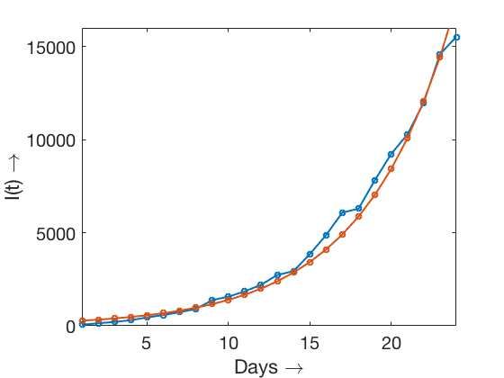
1     SIR model
The classical suspeceptible-infected-recovered (SIR) model in epidemiology [1, 2] allows the
determination of critical condition of disease development in the population irrespective of
total population size over a short period of time. Among many versions of the model, let us
consider the following simplest ODE system:

                                          dS
                                             = −kIS,                                          (1)
                                          dt
                                     dI
                                        = kIS − βI − σI,                                      (2)
                                     dt
                                            dR
                                                 = βI,                                        (3)
                                             dt
for the sizes of the susceptible sub-population S, infected I, and recovered R. The term
kIS describes the disease transmission rate due to the contacts between susceptible and
infected individuals, βI characterizes the rate of recovery of infected, and σI mortality due
to infection only. It is assumed here that recovered individuals do not return to susceptible
class, that is, recovered individuals have immunity against the disease; they cannot become
infected again and cannot infect susceptibles either.
    Analysis of this model is well-known [1, 2] and we will not discuss it here. Since the
coronavirus epidemics is admittedly still in its early stage, let us only determine the condition
of the disease progression at its beginning, i.e. when the number of infected/recovered/dead is
much less than the number of susceptible, and hence S in the model above can be considered
as constant, S ≈ S0 . The equation (2) then turns into the following:

                                      dI
                                         = kIS0 − βI − σI.                                     (4)
                                      dt
so that it splits off the system (1–3) and can be considered separately. It is an ordinary differ-
ential equation with constant coefficients whose solution can readily be found, I(t) = I0 eµt ,
where I0 is the initial number of infected (I0 ≥ 1), i.e. at the time when the infection/disease
was first detected. Substituting this expression into equation (4), we get

                            µ = (kS0 − β − σ) = (β + σ)(R0 − 1),
where the new parameter R0 = kS0 /(β + σ) is called the basic reproduction number. If
R0 > 1, then the number of infected will grow, if R0 < 1 it will decay. Thus, R0 plays
the key role in the epidemics development. In particular, one can change the course of the
disease dynamics by changing R0 . For instance, if measures are introduced that push the
value ofR0 below one (e.g. by making k to decrease), the exponential growth changes to
exponential decay. Interestingly, this is exactly what has happened in South Korea (see
Section 3) after restrictions on daily life were introduced.
    The classical SIR model therefore determines the condition of the disease development
from the comparison of the disease transmission rate with the sum of the recover and death
rates. In the other words, we compare the rates of adding and removal of infected. The model

                                                2
does not account for the incubation period of the disease that was shown to be important
in the case of coronavirus spread: individuals can become infective before showing any
symptoms. A model that allows for the incubation period will be considered in the next
section.
2 Quarantine model
Model. Exceptional measures adopted for the coronavirus infection suggest to introduce
another model of infection development. We consider the sub-population of latently infected
individuals who are already infected but do not show any symptom during the incubation
period. When the incubation period is over, the disease manifests itself with its symptoms,
and the individual is isolated in the quarantine where he/she cannot infect the others. Under
these assumptions, instead of system (1)-(3) we have
dS
= −kI(t)S(t), (1)
dt
dI
= kI(t)S(t) − kI(t − τ )S(t − τ ), (2)
dt
where I is the sub-population of latently infected individuals, τ is the incubation period. The
second term in the right-hand side of equation (2) corresponds to the individuals infected
at time t − τ . Their incubation period is finished at time t, and they are put to quarantine.
As a result they can not speard infection anymore.
Solution. As before, we approximate S(t) ≈ S0 , S(t − τ ) ≈ S0 as τ is not large, and
replace equation (2) by the equation
dI
= kI(t)S0 − kI(t − τ )S0 . (3)
dt
Substituting I(t) = I0 eµt in above equation, we get
µ = kS0 (1 − e−µτ ). (4)
This equation has solution µ = 0 for all values of parameters. Besides this solution, it can
have a positive or a negative solution µ. The function f (µ) = kS0 (1 − e−µτ ) is an increasing
function with the asymptotic limit kS0 at infinity. The sign of the solution is determined by
the derivative f ′ (0). If f ′ (0) > 1, then there is a positive solution (Figure 1), if f ′ (0) < 1, the
solution is negative. In terms of the basic reproduction number R0 = kS0 τ , the condition
is similar as for the SIR model. However, the meaning of this parameter is different. It
characterizes the total infection rate during the incubation period and not its ratio with the
rates of recover and death.
With the notation µ̂ = µ/(kS0 ), we can write equation (4) as follows:
µ̂ = 1 − e−R0 µ̂ (5)
Its solution depends on the single parameter R0 .
3Figure 1: Graphical solution of equation (4), µ = f (µ) with the values of parameters: τ = 1,
kS0 = 2 (blue curve) and kS0 = 0.4 (red curve).
Public health. In the absence of vaccination and lack of effective treatment, the only way
to influence the disease development is to act on the basic reproduction number R0 = kS0 τ ,
that is to decrease the value of the parameter k quantifying the disease transmission rate
by the infected individuals (among which the symptoms are not prominent yet). Note S0
is a characteristic of the given population and τ is the property of the disease, therefore
neither of them is controllable. However, parameter k depends on the human mobility and
the social distance and can be changed. If in the beginning of the disease development k >
1/(S0 τ ), that is each infected individual contaminate in average more than one susceptible
individual during the incubation period, then the number of newly infected individuals will
grow exponentially. If, at some moment of time, measures restricting potential contacts
between infected and susceptible individuals are introduced - the quarantine, then k can
become less than the critical value, and the number of newly infected individuals will start
decaying exponentially, thus resulting in a transition between the growing and decaying
exponentials.
3 Data
We used the data from [4] showing the total number of infected individuals and daily cases
in different countries and worldwide. Across the world, daily cases clearly show two-mode
dynamics such as in China (growth-decay) and Europe (growth). There are periods of
exponential growth, decay and re-growth. The origin of the outbreak on February 12 (in
China) is not clear yet. It may be related to the method of data collection. Daily reported
cases curves in China and South Korea correspond to the growth-decay dynamics. The daily
new cases curves for France, Germany, Italy, Spain, USA correspond to the growth mode.
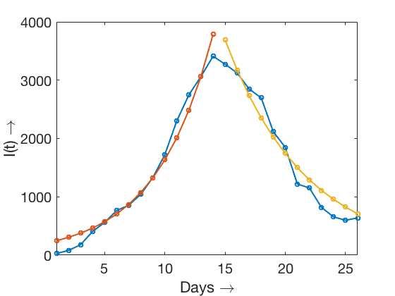
Note that the data on daily reported cases do not exactly correspond to the variable
4I(t). The latter represents a sum of daily cases during the incubation period. Taking into
consideration that the incubation period to be of 5 days, we therefore obtain the graphs
for the latently infected individuals. We observe growth-decay dynamics for South Korea
(Figure 2, left) and growth dynamics in Italy (Figure 2, right).
Figure 2: Latently infected individuals obtained as a sum of daily cases during the incubation
period: (left) South Korea, the growing branch is approximated by the exponential 200e0.21x ,
decaying exponential by 35 · 103 e−0.15x ; (Right) Italy, the data curve is approximated by the
exponential 230e0.18x . In both cases, the value τ = 5 days is used.
Fitting the data allows us to determine the basic reproduction number from equation (5).
For South Korea, R0 = 1.123 on the growing branch and R0 = 0.932 on the decaying branch.
For Italy, R0 = 1.103. We mention here that the basic reproduction number depends on the
incubation period.
4 Discussion
Our model confirms the efficiency of the approach to stop the disease spread by the limiting
the number of contacts between the individuals through quarantine of infected individuals.
This is quite obvious in theory, with the help of the simplest model formulation, but difficult
in practice. Success of the strategy also depends upon the appropriate time of implementa-
tion. Experience of China and South Korea shows that the peak of infection (maximum of
newly reported cases on daily basis) is reached about 10 days after adopting serious restric-
tive measures. The number of infection increased during this time in 10-20 times. In Italy
10 days after the universities and schools were closed (March 4) the peak of infection does
not seem to be reached, and exponential growth continues.
Moreover, the exponential growth rate of the total number of infected in China and in
South Korea observed before the adopted measures (January 25 and February 22, respec-
tively) rapidly changed to a slower growth rate afterward (Figure 3). Similar situation is
observed in Iran though the information about adopted measures is not fully available yet.
5However, in Italy the exponential growth rate does not change up to March 4. This can be
an indication that the introduced measures are not sufficient or that they are not respected
by local people.
Figure 3: Total number of infected in the logarithmic scale. In South Korea (top), the
exponential growth rate (linear growth in this scale) before February 22 is replaced by a
slower growth after this date. In Italy (bottom), the exponential growth rate (linear growth
in this scale) after March 4 does not change.
Limitations of the model. The model has a number of obvious limitations. It takes into
account only the beginning of the disease development where the number of susceptibles can
be considered as constant. Arguably, it is a good approximation if the disease propagation
is stopped/regulated when the number of infected is relatively small compared to the total
population or the focus is on the early stages of the disease development.
Next, and perhaps mode importantly, the model does not take into account the spatial
distribution of infected and their displacement. In this case, instead of equation (3) one has
to consider a model with an explicit space, for instance the following equation:
∂I(x, t) ∂ 2 I(x, t)
=δ + kI(x, t)S0 − kI(x, t − τ )S0 , (6)
∂t ∂x2
where I and S0 now have the meaning of the corresponding densities insread of sizes and
the diffusion term describes small-scale random motion of the individuals with intensity δ
(neglecting long-distance jumps).
In the case where neither of S0 , k and τ depend on space, Eq. (6) can be reduced
to the nonspatial model. Considering, for simplicity, the unbounded space (or a bounded
interval
R∞ with no-flux boundary conditions), we introduce the total size of infected as J(t) =
−∞
I(x, t)dx. Integrating equation (6) with respect to x, for variable J we then obtain an
equation similar to (3).
However, the spatially averaged model does not describe the dynamics in case some of the
parameters depend on space. For instance, if there are two different patches of the disease
development with different basic reproduction numbers, then the disease can be eradicated
in the first patch due to the imposed restrictions but it can give a new outbreak in another
patch if the restrictions are not adopted there or they are not sufficient. This situation is
observed in Europe where the disease progresses exponentially while it is already slowed
down in China. Hence, in some cases, a multi-patch model should be considered with some
6connectivity between the patches at least for some time period. Also, the human movement
can follow a pattern more complicated than is given by the Fickian diffusion, e.g. to follow
the network made by connections between large airports.
Another important limitation of the model is related to the assumption of a single in-
cubation period. According to the available data that are somewhat contradictory and far
from complete, it is possible that there are different incubation periods or maybe the whole
spectrum of incubation periods from several days up to four weeks. The distributed delay
models are more appropriate in this case.
Finally, we mention virus mutations that can have a strong influence on the disease
progression and treatment [3]. At the moment, there are no available data on mutations of
coronavirus, it will take some time before this aspect can be convincingly confirmed or ruled
out.
Acknowledgements
The first author acknowledges the IHES visiting program during which this work was done.
The work was supported by the Ministry of Science and Education of Russian Federation,
project number FSSF-2020-0018, and by the French-Russian program PRC2307.
References
[1] H. W. Hethcote. The Mathematics of Infectious Diseases. SIAM Review 42 (2000),
599653.
[2] J. Murray. Mathematical biology. Volume 1. Third edition, Springer-Verlag, Heidelberg,
2002.
[3] N. Bessonov, G. Bocharov, C. C. Leon, V. Popov, V. Volpert. Genotype dependent
virus distribution and competition of virus strains. Memocs, 2020, in press.
[4] Worldometer: https://www.worldometers.info/coronavirus/
7You can also read