Optimal capital ratios for banks in the euro area - CPB.nl
←
→
Page content transcription
If your browser does not render page correctly, please read the page content below
Optimal capital ratios for
banks in the euro area

Based on a cost-benefit analysis,   The optimum varies greatly
we find optimal risk-weighted       between euro area Member
bank capital ratios in the euro     States. We find lower estimates
area between 15 and 30 percent.     for Member States with a more
The estimated optimum in all        stable economy and a banking
cases is higher than the current    sector that can easily attract
Basel III minimum requirements.     funding.
More capital for banks can lead
to higher lending rates on the
one hand, but also to better
absorption of financial shocks
and mitigating banking crises on
the other.                                         CPB Discussion Paper
                                                 Beau Soederhuizen, Bert Kramer,
                                               Harro van Heuvelen, Rob Luginbuhl

                                                                     September 2021

                                              Doi: https://doi.org/10.34932/yy4h-xp73
Optimal capital ratios for banks in the euro
area
Beau Soederhuizen∗ & Bert Kramer & Gerrit Hugo van Heuvelen & Rob
Luginbuhl
CPB Netherlands Bureau for Economic Policy Analysis
September 6, 2021
Abstract
In this paper we estimate the optimal level of capital for banks in the euro area. Higher
bank capital requirements may be socially costly, as rising funding costs might result in
higher lending rates. On the other hand, if increasing bank capital is socially costly, so
too is not raising bank capital sufficiently. Reserves help banks absorb financial shocks and
thereby reduces the likelihood of banking crises. Our baseline estimates show an optimal risk-
weighted capital ratio of around 22%. Alternative estimates by varying assumptions yield a
range of optimal ratios between 15% and 30%. Despite this considerable spread, this means
that the estimated optimum is higher than the current Basel III minimum requirements in
all cases. We also find substantial heterogeneity across member states. Optimal ratios range
from 27% for banks in Cyprus to as low as 8% in Belgium. This suggests that optimal ratios
are likely inversely related to the resilience of national economies and the ease with which
banks in different member states can raise capital.
Key words: Bank regulation, capital structure, macroprudential policy.
JEL classification: C33, C54, E44 , G15, G21.
∗
Corresponding author: b.soederhuizen@cpb.nl.
We would like to thank Bram Hendriks for helpful comments.1 Introduction
Bank capital provides an important buffer to help absorb financial shocks. This, in turn, helps
to stabilize the real economy. Following the Great Recession, policymakers and academics have
debated about the level of bank capitalization needed to safeguard the economy, because an
international banking crisis played a central role during the onset of the crisis (see, e.g., Admati
et al., 2010; Meh & Moran, 2010). In the euro area, the role of banks was tested a second time
during the Euro crisis.
Prior to the financial crisis, reforms on banking supervision and regulation were already
internationally organized, but this intensified after the recent crises episodes (Kapstein, 1989;
Schoenmaker, 2013; Penikas, 2015). In 1988 a risk-weighing scheme was introduced by the
Basel I reform, in order to take the differences in risk of asset classes into account (BIS, 1988).
The minimum required capital was set at 8% of risk-weighted assets.1 Bank regulation was
tightened internationally by the Basel II capital accord in 2006 (BIS, 2006). In this accord,
capital adequacy requirements were set and the framework of risk-weighted assets amended.
Additional supervisory review was strengthened, and banks had to disclose more information
to ensure market discipline. The Basel III reforms (BIS, 2010b) have set the minimum risk-
weighted capital requirement higher in response to the deficiencies in financial regulation during
the crisis and to strengthen to shock absorbing capacity of banks, exemplified by a minimum of
12.5% for Global Systemically Important Banks (G-SIBs).2
However, higher bank capital requirements may have a negative impact on credit supply and
therefore the economy, as rising funding costs might result in higher lending rates (and thus
lower lending volumes, see e.g. Aiyar et al., 2016 and Meeks, 2017). If this is the case, then
raising the capital requirements would be socially costly. On the other hand, if increasing bank
capital is socially costly, so too is not raising bank capital sufficiently. Reserves help banks
absorb financial shocks and thereby reduces the likelihood of banking crises. Insufficient capital
thus poses a risk to the financial sector and the economy as a whole.
In this paper we provide estimates of the optimal level of bank capital for banks in the
euro area by weighing the costs against the benefits of higher reserve requirements. To our
knowledge, these represent the first empirical estimates for the euro area as a whole. We also
obtain estimates for individual euro area countries.
Our baseline largely follows the analysis of optimal bank leverage for the United Kingdom in
Miles et al. (2013), hereafter referred to as Miles. Our multi-country approach, however, allows
us to extend our analysis further to investigate whether there are differences in the optimal level
1
That is, the ratio between total capital and risk-weighted assets. Before the introduction of this framework,
leverage ratios (total assets over total capital) were most commonly used in supervision.
2
Capital ratios of 12.5% core capital relative to risk-weighted assets often implies only around 4-5% unweighted.
2of bank capital caused either by differences in the resilience of the Euro member states’ banking
sectors, or by differences in the levels of financial frictions across Euro member countries.
Our results show an optimal level of risk-weighted capital for banks in the euro area centers
around 22%. This outcome is fairly robust to several sensitivity checks, and suggests that
optimal capital ratios are in all cases higher than the current Basel III minimum requirements.
Additionally, it indicates that European banks require higher reserves than they currently hold.
Other studies for the UK and US, and one theoretical study for the euro area, find optimal ratios
ranging from around 10% to 25%. We will elaborate on the differences in these studies in the
next section. When exploring heterogeneities between member states, we find the optimal ratio
to range between 27% in Cyprus to 8% in Belgium. This finding indicates that optimal ratios
are inversely related to the resilience of national economies and the ease with which banks in
different member states can raise capital.
The remainder of the paper is structured as follows. Section 2 provides a review of the
literature, and Section 3 places our study in a historic perspective of bank reforms and crises.
Section 4 presents the empirical methodology, and describes the data we use in our analysis. In
Section 5 we discuss our baseline results. In Section 6 we present our robustness checks. Finally,
in Section 7 we end with some concluding remarks.
2 Literature review
The body of empirical literature on optimal bank capital is modest. Birn et al. (2020) provide
a valuable overview. Our contribution to the existing literature is twofold. First, we provide
empirical estimates for the euro area. To our knowledge, we are the first to take on this task.
Second, due to the granularity of our data we are also able to provide estimates for individual
member states.
The seminal paper on optimal bank capital is by Admati et al. (2010). In this work the
authors advocate for higher capital ratios, because, they argue, attracting more capital is not
socially expensive. They argue that high leverage (i.e. weak capitalization) actually makes banks
more inefficient and poses risks created by the expectation of bailouts. The authors, however, do
not provide empirical estimates of optimal ratios, but nonetheless argue that unweighted capital
ratios be increased to around 20% to 30%.
The Basel Committee on Banking Supervision (BCBS) delivered an empirical assessment of
the impact of measures to strengthen the position of banks (BIS, 2010a). The analysis relies on
the trade-off between the benefits of higher capital ratios, in terms of reducing the probability
of a crisis and the amplitude of GDP variability, and the costs, via increased lending rates.
For estimating benefits, they consider both a top-down approach, using country level data to
estimate the relation between crises and bank capital, and a bottom-up approach, estimating
3the relation between capital and default risk on a bank level and then extrapolating this to the
country level. The analysis considers other regulation constant, except for some allowance for
liquidity regulation. In their model they take representative banks from 13 countries over the
period 1993 to 2007.3 Ultimately, they find optimal risk-weighted ratios of between 10% and
15% depending on the extent to which permanent output effects are assumed to follow from a
banking crisis.
For a subset of BCBS members, Fender & Lewrick (2016) update the BIS (2010a) framework
with a new regulatory environment, including more restrictive capital definitions, more strin-
gent requirements for the calculation of risk-weighted assets, liquidity regulation, and capital
surcharges for Global Systemically Important Banks (G-SIBs). Also they use historical data in
their estimations of costs and benefits. They find optimal ratios of between 10% to 11% for
Core Equity Tier 1 ratios (CET1). Barrell et al. (2009), Bank of Canada (2010) and Kato et al.
(2010) provide other early assessments of the merits of bank capital, but do not estimate optimal
ratios.
In Miles the authors were the first to estimate optimal risk-weighted ratios for banks in
a single country. They estimate optimal risk-weighted capital ratios for banks in the United
Kingdom (UK) based on data from 1992 to 2010. They use the bottom-up approach in estimating
the benefits of bank capital, with a one-to-one relation between bank assets and permanent
output effects, and rely on the volatility of the entire economy to prevent with bank capital
instead of only with a financial nature. Regarding costs, they use a structural model to relate
changes in banks’ funding costs to social costs, including a Modigliani-Miller effect of 45%. Their
cost-benefit analysis of acquiring more capital results in optimal ratios in the range of 16% to
20%.
In the framework of BIS (2010a), but estimating the model for banks in the UK, Schanz
et al. (2011) find ratios to be between 10% to 15%. Brooke et al. (2015) provide estimates
for the UK as well, but take a wider perspective on the shock absorbing capacity of banks
by considering the Total Loss Absorbing Capacity (TLAC). Additionally, they assume that a
credible resolution regime lowers the costs of future banking crises, due to effective action by
regulators. They also use a combination of semi-structural models in which more bank capital
reduces real investments, and in turn potential output. With a full-pass trough of funding costs
to customers, they find optimal ratios in the range of 10% to 14%.
In a study on optimal capital ratios for banks in the United States (US), Barth & Miller
(2018) find an optimal baseline estimate of 19%. They estimate a Modigliani-Miller effect of zero
in their calculations of the costs of bank capital, and use the top-down approach for estimating
3
Banks from the following countries are included in the analysis: Australia, Canada, France, Germany, Italy,
Japan, Korea, Mexico, the Netherlands, Spain, Switzerland, the United Kingdom and the United States.
4marginal benefits. The Federal Reserve Bank of Minneapolis (2017) use a model to convert
nonperforming loans into capital losses, and then estimate the marginal benefit of avoiding a
crisis through additional capital. Furthermore, they take the FRB/US macromodel to estimate
the social costs of additional bank capital via lending rates. They derive an optimal ratio
of 23.5%. Combining an estimate for the short- and long-term costs of a banking crisis, and
the same approach for costs as Federal Reserve Bank of Minneapolis (2017), Firestone et al.
(2017) find optimal ratios of between 13% to 25%. Using estimates for the US, with a top-down
approach for benefits and a different CAPM approach than Miles et al. (2013), but extending
the results also to Japan and Western Europe by extrapolation, Cline (2017) finds optimal core
capital ratios between 12-14%. Finally, using DSGE models to estimate the social costs of a
banking crisis Almenberg et al. (2017) find optimal ratios for Swedish banks of between 10% to
24% of core capital.
Most previous studies, like Miles or Barth & Miller (2018), model an inverse relation between
bank capital and the likelihood of a banking crisis, whilst assuming that the cost of a banking
crisis is independent of the level of bank capital. This is also our approach to modeling the
marginal benefits of bank capital. Recent work by Jordà et al. (2021), however, shows that bank
capital is unrelated to the likelihood of banking crises for the period 1870-2015, but that the
severity of banking crises’ does decrease with bank capital. This suggests that an alternative
way to view the benefits of bank capital is not in their role in making crises less likely but in
making them less costly. In either view, there are social benefits to increasing bank capital which
can be weighed against its costs.
The only study with a specific focus on optimal capital ratios for European banks is by
Mendicino et al. (2020). Using a theoretical model, the authors focus on the twin risks from
defaultable loans by clients and from defaults by banks. Calibrating the model to the European
banking sector, they ultimately find an optimal ratio of 15% to avert twin crises.
3 Euro area banking reforms and crises
Europe has a long history of banking crises, dating back at least to the banking crisis in Am-
sterdam in 1763 with the collapse of two substantial banks; subsequently, financial uncertainty
spread to banks in Germany and Scandinavia (Quinn & Roberds, 2015). Thereafter, several
banking crises followed, mainly due to the growing role of banks in the financial sector of Eu-
rope. The dark grey shaded areas in Figure 1 show that the euro are faced banking crises on
multiple occasions and often in prolonged subsequent periods (the dating of banking crisis is
based on Reinhart & Rogoff, 2009 and Laeven & Valencia, 2012). The light shaded areas show
crisis periods for a single European country. A substantial drop in GDP growth can be seen in
the same period, displaying how banks and the real economy are inextricably intertwined. This
5relation runs both ways: banking crises can cause damage to the real economy, but, vice versa,
real economic shocks can also be a driver of banking crises.
Three major periods of banking crises stand out, with the most prominent periods of crisis
being the Great Financial Crisis of 2007/08 and the following Euro crisis, during which average
GDP of European countries declined by roughly 7 percent. Another period of banking crises
occurred in the early 90s in tandem with the European Monetary System (EMS) crisis, with
banking crises in Italy, Finland, Greece and France (Reinhart & Rogoff, 2009). In these countries,
GDP declined accordingly by a little over 4.5 percent. In the late 70s the banking sectors in
Germany and Spain faced considerable financial stress in the wake of the oil crisis; for Spain,
this stress lasted until the early 80s (see e.g., Caprio & Klingebiel, 1996 and Caprio, 2003). In
the early 80s also some Dutch mortgage banks faced bankruptcies. In this period, GDP growth
in the euro area fell from roughly 5 percent to 0 percent.
Figure 1: Periods of crisis in European countries since 1950
.1
1
.05
Real GDP growth
Crisis
-.05
-.1 0
0
1950 1960 1970 1980 1990 2000 2010 2020
year
Crisis period, One Country
Crisis period, Multiple Countries
Real GDP growth
Note: The blue line represents the average of GDP growth for European countries
according to their 2020 membership to the EMU. GDP growth is based on the Mad-
disson dataset. Crisis periods are derived from the Reinhart & Rogoff (2009) and
Laeven & Valencia (2012) databases.
Before these crises, discussions were initiated on the integration of European banking regu-
lation and supervision. The European Commission launched these discussions in 1965 (see, e.g.,
Mourlon-Druol, 2016). In 1969, the group ‘Coordination of Banking Legislations’ reiterated
discussions on the harmonization of banking sector supervision and regulation, without concrete
6results in terms of harmonizing bank regulation. Eventually in 1986 the Single European Act
was accepted, which was to create a single market within the European Union and commence
banking sector coordination. Finally, the process of integrating the European banking sector
reached a crucial stage with the creation of the single currency with the Maastricht Treaty of
1992 and the approval and implementation of the Financial Services Action Plan in 1999.
The financial crisis of 2007/08 and European sovereign debt crisis of 2010 raised the risk of
contamination of financial uncertainty among European countries. To this end, the European
Central Bank (ECB) conducted the first of several EU-wide stress tests in 2009 to evaluate the
resilience of the European banking sector.4 In 2011, the European Banking Authority (EBA)
established a European oversight body for the banking sector. With the Banking Union roadmap
of 2012, the Single Supervisory Mechanism (SSM) and Single Resolution Mechanism (SRM)
were created (see, e.g., Kern, 2015; Quaglia, 2010; Howarth & Quaglia, 2013). To organize a
structured resolution scheme for banks with additional funding, the Single Resolution Fund was
set up in 2015 (gradually being filled until 2024).
In light of the developments concerning crisis episodes and regulatory changes, leverage ratios
(total assets/capital) for banks in the euro area fell from around 30 in 1999 to close to 16 in
2019 (see Figure 2).5 Over time banks improved their capital position, creating a larger buffer
to absorb financial shocks. A large spike can be observed in 2007-08 due to the financial crisis
depleting bank reserves. As the current international standard for macroprudential policy is
risk-weighted capital ratios, we now turn to the most recent capitalization of banks in the euro
area. At the end of our sample, December 2019, the average common equity tier-1 ratio for all
banks in our dataset stands at roughly 16%. For individual member states, the average ranges
from over 12% in Portugal to 22% in Belgium, which are on average close to or above the 12.5%
minimum required by Basel III standards for systemic banks. The union- and country averages
are displayed in Appendix B.
4
Since then, the ECB, and later the European Banking Authority (EBA), conducted six EU-wide stresstests,
in 2010, 2011, 2014, 2016, 2018 and 2020.
5
Due to data availability, we display leverage ratios instead of risk-weighted capital ratios. Accounting stan-
dards required banks to report leverage ratios, and not necessarily risk-weighted capital ratios. This is also
the reason to use leverage ratios in our estimation procedure, as will be presented in Section 4. Eventually we
will translate our outcomes to risk-weighted capital ratios in order to match with the current macroprudential
standard.
7Figure 2: Leverage ratios of banks in the euro area
35
30
Leverage Ratio
25
20
15
2000h1 2005h1 2010h1 2015h1 2020h1
Note: The blue line represents the average of banks in the euro area in our sample
over 1999-2019. See Section 4.1 for a description of our dataset.
4 The costs and benefits of bank capital
Informed decisions about banking sector harmonization in the EMU are dependent on estimates
of the optimal bank capital ratios. Stronger capitalized banks benefit from more shock absorbing
capacity, reducing the probability and impact of potential future banking crises. Conversely,
raising more capital may be costly, both for banks and for the society. In this section, we will
investigate the costs and benefits of requiring more capital for European banks. Our cost-benefit
analysis is based on Miles, which we reproduce and extend here to the European setting. To
perform an analysis on the optimal level of bank capital, we need to find an expression for the
present discounted value of the marginal cost of bank capital and one for the marginal benefit.6
4.1 Costs
The channel through which the costs of bank capital affect the real economy involves a sequence
of economic effects. In the first instance, raising bank capital can lead to increasing funding
costs for banks. We describe the methodology and estimation outcomes of this step in Section
6
Throughout our analysis, we assume all other factors are held constant, including other macroprudential
policy instruments. This means we disregard potential interactions of bank capital with instruments such as
liquidity requirements or changes in bank resolution policy. We also do not take into account the impact of
capital requirements on the risk incentives of banks, and the competition across banks. Both can have an effect
on the marginal costs and benefits of bank equity (for this, see e.g. Gersbach, 2013).
84.1.1. As banks are financial intermediaries, they can pass this increase in costs on in the form
of higher lending rates. This in turn leads to less credit provision, resulting in lower economic
activity. Section 4.1.2 describes the empirical approach and outcomes for the social costs of
acquiring bank capital. For the estimation procedure, we make use of leverage ratios due to
data availability, but to make the translation to the current Basel III standard for minimum
required risk-weighted capital we ultimately convert the outcomes to risk-weighted capital ratios.
4.1.1 Costs for banks
To begin with, we derive the costs of acquiring capital funding for banks. For this step, we rely
on the Capital Assets Pricing Model (CAPM) to derive the Weighted Average Cost of Capital
(WACC) for banks’ funding decisions. Equation (1) shows the WACC relationship between the
return of equity, Re , and the return on (risk-free) debt, Rd , for the respective equity, E, and
debt, D, financing relative to the total funding, D + E. Tax advantages for debt funding might
affect funding structures of banks. As the degree to which this effect affects bank funding costs
is unclear (see, e.g., Auerbach, 2002), we set τ equal to zero in our baseline. This also serves
as an upper bound on the WACC, as tax advantages would result in a lowering of marginal
costs. Later on, in Section 5, we will present the lower bound of our estimates by using national
corporate tax rates. The WACC is expressed as follows:
E E
W ACC = Re + (1 − τ )Rd (1 − ) (1)
D+E D+E
The costs of raising bank capital therefore relies on the return investors demand for providing
equity funding. The return on equity, Re , can be approximated by estimating the equation, using
CAPM:
Re = Rf + βe Rp (2)
in which the return on equity relies on the risk free rate, Rf , the market equity risk premium,
Rp , and the equity beta, βe . The equity beta thus captures the responsiveness of a bank’s return
on equity to national financial market development. For the risk-free rate we take the average
10-year government bond rate of euro area member states, and for the risk-premium we use the
estimate for the average of the euro area from Absolute Strategy Research (ASR), both obtained
from Datastream for the period 1992-2019. The average risk-free rate is 4.74%, and the average
market equity risk premium 4.11%.7
In addition to the risk-free rate and market equity risk premium, (2) is also dependent on
the equity beta, βe . In the CAPM model, it turns out that βe is itself a function of leverage. To
7
We also consider using the 10-year government bond yields and risk-premiums for individual countries. The
risk-premium is, however, not available for all countries. When unavailable, we have used the average for the euro
Area. We note that the cost estimates are almost identical, these results are available upon request.
9demonstrate this, we start with the original CAPM equation:
E D
βa = βe + βd (3)
D+E D+E
where the total beta of bank assets, βa , is given by the weighted sum of the bank’s equity beta,
βe , and debt beta, βd .
Adopting the approach taken in Miles and Barth & Miller, 2018, we assume that βd is zero
and that the return on debt Rd is therefore equal to the risk-free rate Rf . The existence of deposit
insurance ensures that a bank’s deposit liabilities are close to being risk-free. The assumption
of zero risk for non-deposit debt is less obvious, but in the context of the CAPM, risk-free only
implies the weaker condition that any fluctuation in the value of debt is not correlated with
general market movements: βd = 0.
Now solving (3) for our unknown βe , then yields the equation,
D+E
βe = βa (4)
E
E
This demonstrates that βe is inversely related to a bank’s capital ratio, D+E . If we assume
that βa is constant over time, and if we can obtain a measure for βe , then we can estimate the
relationship between βe and the inverse of leverage. This in turn can be substituted into the
WACC in (1) to obtain costs as a function of leverage. It is from this last result that we can
eventually obtain the marginal cost of leverage.
To derive the WACC equation, we thus need to find estimates for βe and the relationship
with leverage ratios. We therefore now turn to the estimation of the components needed for the
WACC of acquiring additional bank capital. Starting off, to estimate the relationship in (4) we
require the equity betas of banks. As these values are not directly observed, we estimate them
using the market model, relating the daily changes in the share price of bank i at time t to the
respective national stock market j on which they are listed (see for example Baker & Wurgler,
2015). To estimate this relationship, we use daily stock prices from Refinitiv Datastream. The
market model is given by:
∆Sit = βe,it ∆Sjt + it (5)
After estimation of equation (5), we take bi-annual averages of the equity betas by bank to
match the frequency of leverage ratios. In total we have 87 euro area banks in our sample over the
period 1992-2019, which have at least 10 observations for both variables.8 We require a minimum
of 10 observations per bank to ensure that our estimates are not primarily representative for a
8
Several euro area banks either have no stock listing or do not have data on leverage ratios publicly available.
Therefore, we miss Latvia, Luxembourg, and Slovenia in the sample.
10specific time period. We use data on a bi-annual basis to increase the number of observations.9
The leverage ratio is expressed as ( D+E
E ), which implies that higher bank leverage ratios are
associated with lower capital ratios, as we saw earlier in (4). In Appendix A we list the banks
in our sample by country.
We note that in some cases a small number of banks show extreme levels of either bank
equity estimates or leverage ratios. As a result, we omit observations that are more than 4
standard deviations from the country mean and remove observations with negative leverage
ratios.10 Table 1 displays the average (bi-annual) bank equity betas and leverage ratio of banks
per country.
Inspecting the values of equity betas, we see that the estimates show considerable dispersion
across countries. The mean ranges from around 0.4 in Finland, France and Austria to 3.6 in
Lithuania. Given this range, it appears that in some cases attracting more capital can have a
considerable impact on funding costs. The average equity beta for banks in the euro area is
0.89. The dispersion in equity betas within countries is even larger: in Lithuania the equity
betas range from -15 to 21.5 but also in Germany the dispersion is quite large from -24 to 2.3.
This large dispersion is mainly driven by small banks with large equity beta estimates.11 This
large within country dispersion is also present in the estimations of, for example, Miles for the
UK and Barth & Miller (2018) for the US.
When we consider average leverage ratios in Table 1, we see that they range from close to
7 in Lithuania to around 28 in Belgium, France and Germany. This would seem to imply that
banks in the latter set of countries have lower capital ratios. Although generally true during
the first part of the sample period, over time banks improved their capital ratios. For example,
German banks had an average leverage ratio of 34 in 1999, yet this decreased to 22 in 2019.
Here too we see a high degree of dispersion among banks within a given country. In Germany,
for example, the leverage ratios vary from 2 for the Umweltbank to above 121 for the Deutsche
Pfandbriefbank. The average leverage ratio for banks in the euro area in our sample is 19.95.
9
Not all banks have publicly available (bi-annual) balance sheet information. For those banks missing bi-annual
data we only consider the year-end observations. For a list of all listed and non-listed banks in Europe, see for
exampe Schoenmaker & Véron (2016).
10
The descriptive statistics show quite some dispersion, both for leverage ratios and equity betas. Using a more
restrictive approach, in which we purge observations with two or three standard deviation from the country mean
yields fairly identical results. These results are available upon request.
11
Excluding these banks with the more restrictive purging method, with 2 or 3 standard deviations from the
country mean, does not change our results.
11Table 1: Descriptive statistics: leverage ratios and equity betas
(D+E)
Leverage Ratio E
Equity Beta, βbe
Countries Mean Min Max N Mean Min Max N
BG 28.02 15.72 71.38 74 1.14 −1.08 3.21 96
CY 14.42 7.92 32.24 44 1.03 −0.58 2.81 96
DE 28.05 2.10 121.34 260 0.74 −23.97 2.25 350
EL 12.78 6.42 35.95 87 1.45 −0.18 3.97 281
EO 12.62 1.41 34.67 26 0.88 0.05 1.87 9
ES 19.81 11.96 54.13 190 1.18 0.11 1.96 273
FN 23.42 3.46 33.91 121 0.43 −1.63 1.76 143
FR 27.92 6.87 58.36 218 0.39 −0.32 2.17 758
IE 18.75 9.07 66.19 98 1.17 −0.80 3.26 134
IT 16.46 2.71 54.00 552 0.82 −0.41 5.03 762
LT 6.94 2.19 18.03 25 3.58 −15.17 21.50 40
MT 12.32 5.24 29.55 64 2.01 −7.25 12.37 116
NL 22.25 13.16 49.50 141 0.82 −0.07 2.52 196
OE 15.89 2.29 51.52 183 0.39 −14.06 10.65 349
PT 16.27 12.61 26.22 26 1.40 0.16 2.45 55
SK 12.95 9.69 21.24 59 2.53 −10.10 22.82 104
EA 19.95 1.41 121.34 2168 0.89 −23.97 22.82 3762
Note: Purging observations with more than 4 standard deviations from the country mean leads to a
drop of a mere 27 observations. BG=Belgium, CY=Cyprus, DE=Germany, EL=Greece, EO=Estonia,
ES=Spain, FN=Finland, FR=France, IE=Ireland, IT=Italy, LT=Lithuania, MT=Malta, NL=the Nether-
lands, OE=Austria, PT=Portugal, SK=Slovakia, EA=euro area average.
ˆ , we can assess the relationship between bank
With the estimates of the equity betas βe,it
equity betas and leverage ratios ( D+E
E , from here noted as λ) as expressed by equation (4). We
estimate this relationship using the following panel fixed effects regression, with bank (αi ) and
period (αt ) fixed effects.12
βd
e,it = a + b λit + αi + αt + µit (6)
where the µit are the residuals, which are components of the equity beta that are not explained
by either the leverage ratio of a bank, or the fixed effects.
As the estimation of equity betas is subject to empirical uncertainty, in section 6 we will
extended the empirical analysis in Miles by performing within-bank block bootstrapping on the
residuals it from (5). We do so because the equity betas are used in equation (6), this uncertainty
12
In our baseline setting, we use bi-annual FE, but using year FE yields similar results. We note that we are
unable to include country effects as they are no longer identified once the model includes bank effects.
12might also feed through to the relationship between leverage ratios and equity betas.13
Before turning to the results of the panel estimations of equation (6), we note that the
econometric literature has shown that the appropriate normalization of fixed effects is essential
when applying the estimated constant parameter, a, in further analysis (Suits, 1984 and Teulings
et al., 2016).14 Therefore, we want to avoid that the normalization by statistical software to
different year or bank observations affects the estimation of a. To solve this, we normalize the
fixed effects to zero and add the mean of the fixed effects to the estimated constant. Papers
focusing on one country, such as Miles, will suffer less from this problem as normalizing to a
different time period or bank by statistical software will occur less frequently. However, even in
the case of a single-country analysis, splitting the sample into two groups in the estimation may
allow the normalization to different time periods or banks to influence the constant substantially.
For example, Barth & Miller (2018) perform such a split to obtain estimates for both large and
small banks. Not correcting for this normalization might complicate the use of a constant in
further analysis.
In Table 2, we report the estimates we obtain based on (6), using the appropriate normaliza-
tion. In addition to the panel FE specification, we also estimate the model with random effects.
The Hausman test shows that the FE specification is statistically preferred. We therefore opt
for using the FE based estimate in our baseline for the remainder of the paper.15
We can then substitute βe out of (2) using the estimated intercept â, including the normal-
ization, as well as the estimated coefficient for leverage, b̂. The estimated coefficient â reflects
the constant part of the equity beta, and hence captures the time-invariant impact of the risk
exposure of the bank to equity for its return on equity. The time-varying impact of a bank’s
capitalization on the return on equity is captured by b̂. At the same time, this reflects the extent
to which an MM-offset is present, as it displays the extent to which changes in capital will lead
to a change in the bank’s funding costs through equity. The substitution of βe allows us to
rewrite (2) as a function of leverage, λ, and the observed risk-free rate, Rf , and market equity
risk premium, Rp :
Re = Rf + (â + b̂ λ)Rp (7)
Like Barth & Miller (2018), we do not consider the presence of a Modigliani-Miller offset,
13
The residuals are redrawn 1000 times in random order, within each bank and by each half-year period. This is
thus a within-bank block bootstrapping approach. The procedure is chosen as some time periods have substantial
more uncertainty then others, e.g. during the financial crisis.
14
That is, choosing a different time period in a panel fixed effect estimation procedure may result in a substantial
difference in the estimated constant parameter if not normalized appropriately. This could then have a sizable
impact on the calculation of the cost of additional bank capital.
15
Even though the Hausman test statistically rules out the Panel RE estimator, we opt for analyzing the
sensitivity of our results to using either the Panel RE or Panel OLS estimators. Results are fairly similar using
the other estimators, and are available upon request.
13Table 2: Estimates from panel regressions
All Banks
Pooled OLS Fixed Effects Random Effects
Leverage, b̂ 0.006 0.000 0.002
[0.006] [0.002] [0.004]
Intercept, â 1.314 1.034 1.353
[0.177] [0.051] [0.165]
N 2092 2092 2092
Rsquare Within 0.035 0.034
Rsquare Between 0.007 0.390
Rsquare Overall 0.176 0.019 0.169
Hausman p-value 0.002
which means that we do not restrict the effect of b̂, whilst Miles considers an MM-offset of 45%.
We note that we can construct plausible bounds for b̂ based on the degree to which we assume
that the Modigliani-Miller (MM, Modigliani & Miller, 1958) effect holds. The MM-theory states
that the costs of raising additional equity is exactly offset by the resulting decline in the interest
rate, Re caused by the lower perceived riskiness of bank equity. This implies that Re in (2) and
(7) will fall whenever leverage declines. By a MM-offset of 100%, this decline in Re leaves the
WACC in (1) unchanged. In this case b̂ > 0 and is large enough to ensure that Re sufficiently
declines to leave costs unchanged. This implies a reasonable upper bound on the value of Re .
By an MM-offset of 0%, we might expect that Re does not respond to leverage, with the
result that total capital costs rise with declining leverage.16 This implies that b̂ = 0, and could
reasonably taken to be a lower bound. In the case of our baseline estimate based on FE, b̂ is
not significantly different from zero.17 This is consistent with the lower bound of b̂ = 0. We
note that the size of the MM-effect has been empirically estimated, for example by European
Central Bank (2011) for large international banks, and has been found to range from 41% to
as much as 73%. The implicit estimates of Kashyap et al. (2010) are close to these estimates,
with an MM-offset ranging between 36% and 64%. These estimates are consistent with b̂ > 0.
Furthermore, while we do obtain positive estimates of b̂ using OLS and RE estimators, these
values are also not significantly different from zero.
Using equation (7), and the average risk-free rate of 4.74%, market equity risk premium of
16
It is however also conceivable that Re actually increases with declining leverage. In this case b̂ < 0.
17
To derive the WACC of acquiring more bank capital, we need an estimate for b̂. Even though b̂ is not
significantly different from zero, it is the best fit to the data, and we will use the panel FE estimators in the
remaining derivations. In Section 6 we will display the results relying on a within-bank block bootstrapping
procedure for equity betas, which include a wide range of b̂ estimates, including statistically significant coefficients,
without affecting the final estimates of optimal capital ratios substantially.
144.11% and leverage of 20 (the euro area average, see Table 1), the return on equity equals 8.98%
for the average of euro area banks. These estimates lie somewhat below those of Miles, which
finds a return on equity of 14.85% for a leverage of 30, but close to those of Barth & Miller
(2018) for a leverage of 25 as they find a return on equity of 8.08% for banks with at least $1bln
in assets and 9.73% for more than $10bln.
From equation (1), with no tax advantage of debt and no MM-offset, we obtain an average
WACC equal to 4.95% when the average euro area bank leverage equals 20, rising to 5.17%
when leverage falls to 10. Again, these estimates are close to those of Miles and Barth & Miller
(2018). The former derives the average WACC to increase from 5.33% for a leverage of 30 to
5.66% for a leverage of 15, where the latter derives an average WACC of 5.19 for a leverage of
25 increasing to 5.71 when leverage falls to 6 23 .
4.1.2 Costs for the economy
In what follows, we relate the WACC of a bank to the macroeconomic implications, through
the lending channel. That is, higher costs of funding via additional bank equity can be passed
on to customers and result in lower credit provision. This, in turn, has a negative impact on
economic activity. Here we report the macroeconomic implications for the average of all euro
area banks in our sample. We first derive the present value GDP effects of a change in leverage
ratios, but eventually convert to the effects due to a change in risk-weighted capital ratios. This
latter instrument is the most prominent instrument used by policymakers internationally to set
minimum capital requirements to banks.
We first determine the effects of a change in the price of capital, Pk , on output, Y . We
then calibrate how the marginal cost of capital is affected by to a change in leverage affects Pk .
This enables us to combine the marginal cost of leverage with the marginal change in output to
obtain the total cost of a change in leverage.
To begin with, we assume that Y is produced via a production function with constant
elasticity of substitution between the two inputs capita, K and labour L. From here, we can
obtain the following expression for the marginal effect of Pk on Y :
∂Y Pk ∂Y K ∂K P ∂P Pk
=
∂Pk Y ∂K Y ∂P K ∂Pk P
Here we have defined the price P to be the relative price of capital to labour: P = Pk /Pl .
This expression relates the elasticity between output and the price of capital to the elasticity
of output with respect to capital, the substitution elasticity between capital and labor, and the
elasticity of relative price to the cost of capital. This combination results in the sensitivity of
15output to the cost of capital. Miles show that this can be rewritten as
∂Y Pk 1
= ασ (8)
∂Pk Y α−1
where α represents the elasticity of output with respect to capital, σ the substitution elasticity
1
between capital and labour, and α−1 is the elasticity of the relative price with respect to the
cost of capital. We use an α of 0.37 (the same calibration is used in Havik et al., 2014 and
European Commission, 2018), and a σ of 0.5. For an overview of the literature on σ estimates
see, e.g., Klump et al., 2012. This parameter setting implies, based on (8) that a 1% increase
in firms’ cost of capital could lead to a reduction in output of 0.29%. In Table 3, we display all
technical assumptions, including those of the production function. In section 6, we check the
sensitivity of our estimates to these and several of the other parameters.
Table 3: Technical Assumptions
Assumption Parameter Value
Share of bank lending Ω 0.45
Substitution elasticity σ 0.50
Share of capital α 0.37
Discount rate δ 0.025
CET1 ratio CET1 0.95
RWA Basel conversion RWAconv 1.25
Now we can combine the channels to derive the present value GDP effects of additional bank
capital. The cost of additional capital is given by the difference in WACC due to the increase
(decrease) in capital (leverage) multiplied by the cost of capital for firms (CoC, that is the risk-
free rate plus the market equity risk premium). This is then multiplied by the share of bank
financing for non-financial corporations, Ω, which we calibrate to be 45% (see for Europe e.g.,
Adalid et al., 2020).18 This in turn can be multiplied by the production function elasticities in
(8) to obtain the loss in economic activity as a result of additional bank capital.19 To obtain
the present discounted value, we discount the result by δ:
ασΩ(∆(W ACC) ∗ CoC)
P VGDP = (9)
δ (α − 1)
18
Admittedly, assuming a constant share of bank financing over time and across countries is a simplification.
This share is likely to vary, and could change in response to the actual costs of capital, driving possibly towards
more market financing. Investigating the relationship between the costs of additional bank capital and the share
of bank financing is left for further study.
19
This ensures that we only consider the economic implication of bank costs related to its funding, and not to
other costs such as labor or overhead costs. We do not account for taxes, because they redistribute part of the
social costs, but do not change them.
16Without an MM-offset, the firms cost of capital is likely to increase by a little under 10 bps
(22bps increase in the WACC multiplied by the share of bank lending of 0.45). Assuming that
the cost of capital is around 9% (risk-free rate plus market equity risk premium), this translates
into a increase 0.9% in the cost of capital for firms. Using a discount rate of 2.5%, and the
outcome of (8) this results in a permanent fall in output of around 10% or 1000bps (that is,
(0.9%x0.29%)/2.5%). That is, a capital ratio increase which lowers leverage to half its original
value would lead to a permanent fall in GDP.
The present value of the cost of bank capital should be translated to marginal costs in order
to compare it with the marginal benefits. Therefore, like Miles we divide the P VGDP by the
change in risk-weighted capital. For this, we translate the change in the leverage ratio from 20
(λ1 ) to 10 (λ2 ) to risk-weighted capital.
CET 1 A 1 CET 1 A 1
∆(CapitalRatio) = ( ∗ ∗ )−( ∗ ∗ ) (10)
λ2 RW A RW AConv λ1 RW A RW AConv
We therefore first rescale the leverage ratio, λ, with the ratio of Common Equity Tier-1
capital to Tier-1 capital (CET1). On average, this is 0.95 over our sample, for which a leverage
ratio of 20 (TA over Tier1 capital) corresponds with a leverage ratio of 21 (TA over CET1-
capital). We use assets to Basel II RWA of around 204% in our sample of euro area banks
(A/RWA), and the same conversion factor as Miles of 1.25 to turn Basel II in Basel III RWA
(RWAConv). Together, the change in risk-weighted capital ratios increase from 7.8% (leverage
of 20) to 15.5% (leverage of 10).
Based on the derivation above, which includes some rounding and thus deviates slightly from
our actual derivation, for each 1%-point increase in risk-weighted capital ratios marginal costs
are around 130bps (that is, present value of costs of 1000bps divided by the change of 7.7% in
risk-weighted assets).20 The marginal costs are fairly close to those derived by Miles for banks in
the UK, as they find marginal costs of around 149bps for each 1%-point increase in risk-weighted
capital ratios.
4.2 Benefits
If increasing bank capital is socially costly, so too is not raising bank capital sufficiently. In the
previous section we measure the private costs (to banks) of raising additional capital, and argue
that these carry over to societal costs, by increasing lending costs. The benefits of increasing
20
Admittedly, the empirical approach leads to a marginal cost estimate that is not dependent on the amount
of bank capital. Most likely, banks that hold almost no reserves will face substantially higher funding costs than
banks with plentiful reserves. In Section 6 we explore this potential non-linearity with piece-wise linear estimation
techniques, but due to data availability constraints we are unable to create bins for banks for small ranges of
capital levels (for example, bins for banks with 0-1% capital).
17bank capital occur at a societal or macro level, because higher bank capitalization decreases the
risk of a banking crises. This benefit of raising capital is what we model in this section.
Following the analysis in Miles, we assume that more bank capital, or lower leverage, increases
banks’ ability to absorb macroeconomic shocks. The idea is that recessions lead to business
failures which, in turn, lead to a loss on banks’ loan portfolios. If the aggregate loss on loan
portfolios exceeds the amount of capital that banks hold, a banking crisis ensues. As a result,
higher levels of bank equity reduce the likelihood of a banking crisis.
We assume that there is a one-for-one relation between GDP losses and losses on bank assets.
In other words: a percentage decline in GDP results in the same percentage decline in the total
value of bank assets. A banking crisis then occurs whenever the percentage decline in GDP
exceeds the average bank capital ratio. Miles present evidence in favour of this one-for-one
relation in their Appendix B, which is based both on the Great Financial Crisis and selected
financial crises from the 1990s.21
We formalize this as follows. We denote the probability of a banking crisis by pb , the
percentage lost on bank asset values by la , the percentage change in GDP by y, and the capital
ratio by λ−1 . We then have the following:
pb = prob(la > λ−1 ) (11)
We further assume that la = −y when y < 0, and la = 0 otherwise. If we substitute −y into
this expression, for when y < 0, then we have the following:
pb = prob(y < −λ−1 ) = Fy −λ−1
(12)
where Fy denotes the cumulative density function of y. Note that in the latter expression we
have that y < −λ−1 < 0, so that y < 0 holds. This formalizes our assumption that the benefit
of a lower leverage ratio is to reduce the chance of a banking crisis.
The assumption that a banking crisis occurs whenever the percentage decline in GDP exceeds
the average bank capital ratio is admittedly simplistic, with no risk of a banking crisis until the
threshold drop in GDP is exceeded. It would be arguably more realistic to assume an increasing
risk of a crisis as a function of the size of the decline in GDP. In practice this would produce
a somewhat more smeared out distribution in (4.2) which would not only be dependent on the
distribution of the growth rate of GDP. Implicitly we assume that the distribution of the growth
rate of GDP captures most of this uncertainty. We leave a more nuanced modeling of (4.2) for
21
Note that results do change if this relation is assumed to be different. If GDP shocks induce bank asset losses
that are as a percentage twice as large, the optimal capital ratio will also be twice as large.
18future research.22
4.2.1 The Distribution of GDP growth
To measure the probability of a banking crisis, we require a probability distribution function for
GDP fluctuations. We therefore estimate the probability distribution of fluctuations of GDP per
capita. We deviate from Miles in two respects. Firstly, we allow for, and test for the fitness of,
alternative parametric forms of the distribution of GDP per capita growth. We expand on this
matter in the next few paragraphs. Secondly, we use data for the annual growth of GDP per
capita for EMU member states between 1950 and 2016, taken from the Maddison Project (Bolt,
Jutta and Van Zanden, Jan Luiten, 2014). Given the focus of our study, this seems like the most
relevant sample. We note that Miles calibrate their model based on an international sample of
high income countries, covering the period from 1820 to 2008 annually. This covers a period
that obviously includes a number of catastrophic events such as the World Wars. Whether or
not this longer sample is to be preferred depends on whether or not one believes banking sectors
should be robust to such events. We opt to use a post-war period from 1950 to 2016 as our
baseline sample, and thereby implicitly consider World Wars as lying outside the set of events
which the banking sector should be able to absorb. We also note that our robustness checks
include estimates based on a longer sample period, which includes both World Wars.23
GDP growth is well-known to be fat-tailed, see for example Fagiolo et al. (2008), Gabaix
(2016) and Williams et al. (2017). Additionally, GDP growth may well be asymmetrically
distributed, where large negative shocks are more likely than similarly large growth events. It
is therefore important not to model GDP growth as normally distributed; rather, one requires
a distribution that allows for excess kurtosis as well as left-skewness.
In Miles, the authors opt to capture these characteristics by modelling the GDP growth
distribution as a normal distribution supplemented with two types of shocks. In their model,
GDP growth is normally distributed, with in any year the possible addition of one of two possible
shocks: a c-type or a b-type shock. The c-type shocks are events that involve either the addition
or subtraction of c to the mean of the normal distribution. The addition and subtraction of c
are equally likely. One can think of these events as typical recessions or boom years. On the
other hand, a b-type shock is a more extreme event and always implies the subtraction of b
from the mean of the normal distribution. For this, one can think of a catastrophic event such
22
We note that in (4.2) we also do not explicitly differentiate between measures of leverage based on risk
weighted assets or based on all assets. Here too we are implicitly assuming that this distinction produces an effect
that is only of second order in size.
23
Including the World Wars give more variability to the GDP distribution, and hence more extreme crisis
periods. This might also proxy for other crisis events that origin from outside the banking sector, such as the
COVID-19 pandemic.
19a war or natural disaster. This b-type shock is inspired by Barro’s (2006) hypothesis that asset
prices incorporate small but meaningful risks of disasters. The probabilities of c- and b-type
shocks transpiring are denoted by pc and pb , respectively. GDP growth is therefore assumed to
be generated as follows:
yt = t−1 + ζt−1 , where t ∼ N (γ, σ 2 ) (13)
and P (ζt = 0) = 1 − pc − pb , P (ζt = −b) = pb , P (ζt = −c) = pb /2, P (ζt = c) = pc /2.
Although the distribution of Miles accommodates both the skewness and kurtosis, it comes
with two main drawbacks. Firstly, depending on the parameters, the distribution of GDP growth
may become bi-modal. This is the case with the parametrization found in Miles where b is 35%.
As a result, a GDP-decline of 35% is more likely than one of, say, 20% or 25%. This is not
well supported by the data. Secondly, left-skewness is imposed in this distribution, and only
captured by the b-parameter. A more flexible functional form, which can also match data that
are not left-skewed, is to be preferred if one wants to fit the family of distributions on various
(sub-)samples.
Fagiolo et al. (2008) test to what extent GDP fluctuations can be described by various
families of distributions. Testing a host of families, they reach the conclusion that the so-called
Exponential Power (EP) distribution well describes GDP fluctuations for nearly all OECD-
countries in the post-World War Two era. The density of the EP distribution is presented in
equation 14 and it is characterized by three parameters: m, a, and b. The parameter b is the
shape parameter: lower values of b correspond to distributions with fatter tails. The normal
distribution is nested in the EP-distribution, where b = 2.
1 − 1b | x−m |b
fEP (x; m, a, b) = 1 e
a (14)
2ab1/b Γ(1 + b)
Fagiolo et al. (2008) further test whether the Asymmetric Exponential Power (AEP) distri-
bution outperforms the EP-distribution, and conclude that in general it does not. This AEP is
similar to the EP distribution, but accommodates different parameter values for a and b on the
left and right half of the distribution. We present this distribution in equation 15.
1 x−m b
K −1 e− bl | al | l if xdistributions to the data.24 We then perform a number of Goodness-of-Fit tests to evaluate
whether the data can in fact be described by the distribution at hand. Aside from the sample
of countries, our analysis differs from that of Fagiolo et al. (2008) in two important respects.
Firstly, we use the annual growth rate of GDP per capita, as opposed to the growth rate of
GDP. Secondly, we fit the distributions based on the growth rates from the entire panel, whereas
Fagiolo et al. (2008) fit the distribution for each individual country. Given these differences, we
have opted to explore which distribution best fits the data.
Table 4 presents the outcomes of Goodness-of-Fit tests. The value of each test statistic
is shown with the p-values underneath in parentheses. The three Goodness-of-Fit tests we
perform on all distributions are the Kolmogorov-Smirnov (KS), Cramér-von Mises test (CvM),
and Anderson-Darling (AD) test. For all three tests, the null hypothesis is that the data can be
described by the fitted distribution.
Table 4: Goodness-of-Fit Tests
test
Kolmogorov-Smirnov Cramér-von Mises Anderson-Darling
Distribution (KS) (CvM) (AD)
Asymmetric Exponential Power (AEP) 0.022 0.059 0.423
(0.642) (0.817) (0.825)
Exponential Power (EP) 0.039 0.368 2.785
(0.064) (0.088) (0.035)
Cauchy 0.054 0.681 8.157
(0.003) (0.014) (0.000)
Gaussian 0.104 3.702 22.165
(0.000) (0.000) (0.000)
Lévy-Stable 0.032 0.253 2.126
(0.197) (0.185) (0.078)
Miles 0.030 0.196 1.381
(0.254) (0.275) (0.208)
Note: For all three tests, the null hypothesis is that the data can be described by the fitted distribution.
P-values are shown in parentheses.
The p-values of the Goodness-of-Fit tests indicate that the AEP distribution is best suited
for our sample of data. This is in line with the conclusions of Fagiolo et al. (2008). We therefore
opt to use the AEP distribution in our baseline analysis. For comparability with Miles, we
include their distribution as one of our robustness checks; as Table 4 shows, Miles’ distribution
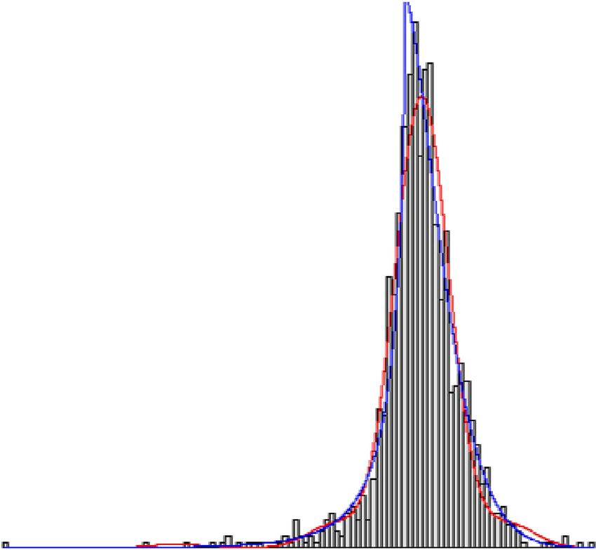
also passes the Goodness-of-Fit tests. In Figure 3, we show the histogram of the growth rates
24
The other distributions we fit are the Gaussian, Cauchy, and Lévy-Stable distributions.
21together with the fitted AEP and Miles densities.
Figure 3: Fitted AEP and Miles Densities and Histrogram
C)
11,0
I I
-0.3 -0.2 -0.1 0.0 0.1 0.2
The AEP fitted density is shown in blue. The fitted Miles density is shown in red.
4.2.2 The Benefit of Averting a Banking Crisis
If a banking crisis can be prevented from occurring, then the loss in output associated with
the crisis can be avoided. This represents the benefit to society of lowering the leverage ratio.
We note that there are presumably other benefits which we could also consider. For example,
lower bank leverage most likely would result in lower deposit insurance premiums for banks,
because the chance of default would be reduced. Such benefits are, however, likely to represent
second order effects, and pale in comparison with the large costs in terms of lost output due to
a banking crisis. As a result, we only consider the present discounted value of lost output due
to a banking crisis in our calculation of the benefits of increased bank capital.
We calibrate the present discounted value of the loss in output due to a banking crisis for
high income economies based on Luginbuhl & Elbourne (2019).25 In their article, the authors
estimate impulse response functions, IRFs, of a banking crisis using the banking crisis dates
25
Their estimated loss is one third smaller than that found in Cerra & Saxena (2008) due to the fact that the
model in Luginbuhl & Elbourne (2019) also accounts for temporary losses caused by the business cycle. Miles
calibrate the cost of a banking crisis based only on the 2008 financial crisis.
22You can also read