OPTIMIZING MACHINE LEARNING MODELS FOR GRANULAR NDFEB MAGNETS BY VERY FAST SIMULATED ANNEALING - NATURE
←
→
Page content transcription
If your browser does not render page correctly, please read the page content below
www.nature.com/scientificreports
OPEN Optimizing machine learning
models for granular NdFeB
magnets by very fast simulated
annealing
Hyeon‑Kyu Park1, Jae‑Hyeok Lee1, Jehyun Lee2* & Sang‑Koog Kim1*
The macroscopic properties of permanent magnets and the resultant performance required for
real implementations are determined by the magnets’ microscopic features. However, earlier
micromagnetic simulations and experimental studies required relatively a lot of work to gain any
complete and comprehensive understanding of the relationships between magnets’ macroscopic
properties and their microstructures. Here, by means of supervised learning, we predict reliable
values of coercivity (μ0Hc) and maximum magnetic energy product (BHmax) of granular NdFeB magnets
according to their microstructural attributes (e.g. inter-grain decoupling, average grain size, and
misalignment of easy axes) based on numerical datasets obtained from micromagnetic simulations.
We conducted several tests of a variety of supervised machine learning (ML) models including
kernel ridge regression (KRR), support vector regression (SVR), and artificial neural network (ANN)
regression. The hyper-parameters of these models were optimized by a very fast simulated annealing
(VFSA) algorithm with an adaptive cooling schedule. In our datasets of randomly generated 1,000
polycrystalline NdFeB cuboids with different microstructural attributes, all of the models yielded
similar results in predicting both μ0Hc and BHmax. Furthermore, some outliers, which deteriorated
the normality of residuals in the prediction of BHmax, were detected and further analyzed. Based on
all of our results, we can conclude that our ML approach combined with micromagnetic simulations
provides a robust framework for optimal design of microstructures for high-performance NdFeB
magnets.
Recently, industrial demands for permanent magnets such as NdFeB (or Nd2Fe14B) are growing due to their
applications to high-performance motors used in electric vehicles (EVs). In particular, NdFeB magnets have
attracted intense interest in both research and industrial fields owing to their unique properties as a hard-
magnetic material, including outstanding maximum magnetic energy product (BHmax), relatively high coerciv-
ity, and lower content of precious rare-earth elements per molecular weight than other hard-magnets such as
SmCo5. Research on NdFeB magnets has progressed rapidly since their discovery in the 1 980s1; the highest
experimentally observed value of BHmax has reached ~ 56 MGOe, close to the theoretically calculated maximum
intrinsic value of 64 M GOe2,3. Nevertheless, much of the study thus far has focused on building up the relation-
ships between macroscopic magnetic properties (e.g. coercivity and BHmax) and microstructural features (e.g. the
thickness of grain b oundaries4, average grain s ize5,6, and the degree of misalignment of easy axes of individual
7
grains ) based on experimental observations and finite-element micromagnetic simulations.
Meanwhile, machine learning (ML) is a set of computational methodologies that are capable of learning and
recognizing patterns and relationships, based on minimization of error (or an optimization of loss function).
Recently, ML-based methods have found great success in the prediction of material properties8, the discovery
of materials9, the design of materials10, as well as in the striking reduction of computation time of electronic
structure calculation11. Application of ML to the fields of hard magnets also has been explored in recent y ears12–15.
For example, Möller et al.12 trained a support vector regression (SVR) model to predict the magnetic material
properties of doped NdFeB with less rare-earth contents by combining the ML method with density functional
1
Nanospinics Laboratory, Department of Materials Science and Engineering, National Creative Research Initiative
Center for Spin Dynamics and Spin‑Wave Devices, Research Institute of Advanced Materials, Seoul National
University, Seoul 151‑744, South Korea. 2Platform Technology Laboratory, Korea Institute of Energy Research, 152
Gajeong‑ro, Yuseong‑gu, Daejeon, South Korea. *email: jehyunlee@kier.re.kr; sangkoog@snu.ac.kr
Scientific Reports | (2021) 11:3792 | https://doi.org/10.1038/s41598-021-83315-9 1
Vol.:(0123456789)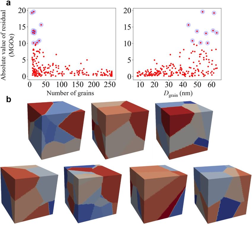
www.nature.com/scientificreports/
Figure 1. Exemplary polycrystalline NdFeB cuboid of 25.9 nm average grain size with grains indicated by
different colors. This figure was created with the open source software ParaView (http://www.paraview.org),
licensed under a Creative Commons Attribution 4.0 License.
theory. Their model was able to predict the material’s intrinsic magnetic properties, including the saturation
magnetization, the anisotropy coefficient, and the Fermi energy, based on given atomic structures with a Pearson
correlation coefficient up to 0.92. Meanwhile, Exl et al.13 utilized a random forest (RF) model in order to char-
acterize the role of microstructural features (e.g. position/size/shape of grains, misalignment of easy axes, etc.)
in the switching of an exemplary permanent magnet. The model was able to provide qualitative and quantita-
tive information on which microstructural feature plays the major/minor role in switching. Gusenbauer et al.14
used an ensemble method combining RF and gradient boosted regression (GBR) models in order to predict the
nucleation field from electron backscatter diffraction (EBSD) images of the surfaces of hard-magnetic MnAl
material. They recommended taking advantage of micromagnetic simulation to see the overall trends in the
heng15 employed an SVR
distribution of nucleation fields or to find weak spots in the microstructure. Further, C
model with hyper-parameters obtained by metaheuristic particle swarm optimization in order to correlate, based
on experimental data, the chemical composition of materials with their macroscopic magnetic properties such
as magnetic remanence, coercivity and BHmax.
However, direct application of ML for prediction of such macroscopic magnetic properties with chemical
compositions involves some risks. In general, the coercivities of polycrystalline NdFeB magnets are heavily
dependent on microstructural factors as described by the phenomenological relation proposed by Kronmüller
and Fähnle5,6. Furthermore, inter-grain decoupling is crucial to determination of the switching mechanism,
whether it is Stoner-Wohlfarth-type coherent r otation16 or Kondorsky-type domain-wall m otion17. Such different
switching mechanisms have been thought to directly impact c oercivities18–20. Decoupling between individual
grains is achieved by spacing out the grains by more than the intrinsic exchange length of bulk NdFeB (~ 1.7 nm),
as realized by doping a trace amount of gallium4. Thus, the potential of ML to accurately predict the macroscopic
properties of NdFeB by employing microstructural attributes needs to be further explored.
In addition, ML models of high accuracy and, at the same time, good quality (i.e. high normality of residual
distributions) are desired. Accuracy is determined by a set of mathematical parameters of ML models, called
hyper-parameters. Conventionally, hyper-parameters are optimized by brute-force techniques such as grid
search21,22 and random search23, which, however, demand laborious try-and-error procedures and are easily
trapped into local minima. Alternatively, simulated annealing is a metaheuristic method that is easy to under-
stand and provides solutions to myriads of optimization p roblems24,25. Like randomized local searching, simu-
lated annealing solves optimization problems by randomly moving from one candidate solution to a neighboring
solution, but with a certain probability that depends on differences in energy and current temperature, the latter
of which is defined by a cooling schedule. Moreover, good quality of models can be assured by analyzing residuals
and quantifying the linearity of their quantile–quantile plots.
In this work, we established a database of 1000 different microstructures of polycrystalline NdFeBs (see
Fig. 1) of 128 nm × 128 nm × 128 nm cuboid geometry using a GPU-accelerated micromagnetic simulation
package. We predicted the macroscopic magnetic properties of coercivity and BHmax by ML models according to
microstructural parameters such as inter-grain exchange stiffness Aint, average grain size Dgrain, and the degree of
misalignment of easy axes of grains σθ. Moreover, we tested a variety of ML models such as kernel ridge regres-
sion (KRR), SVR26,27, and artificial neural network (ANN)28 with their hyper-parameters optimized by a very
fast simulated annealing (VFSA) algorithm that adopts an adaptive cooling schedule. Further, we performed
a residual analysis in order to assure the quality of the models, and we detected some outliers that deteriorate
model quality in the case of BHmax prediction. Our results demonstrate the potential of ML methods for future
design of NdFeB magnet microstructures in cases where the underlying microstructure-property relationships
are not yet clarified.
Scientific Reports | (2021) 11:3792 | https://doi.org/10.1038/s41598-021-83315-9 2
Vol:.(1234567890)
www.nature.com/scientificreports/
Results
Results of micromagnetic simulations. In Fig. 2a,b, the dependences of coercivity (μ0Hc) and BHmax
on reduced parameter aint (= Aint /Aex , where Aex is the exchange stiffness constant), Dgrain, and σθ are displayed
with the corresponding Pearson correlation coefficient (ρ), respectively. Both coercivity and BHmax increase as
σθ decreases with the Pearson correlation coefficients of −0.858 and −0.925. Furthermore, both coercivity and
BHmax had a curvilinear relationship that fits with a third-order polynomial formula with respect to σθ. This
resulted from nucleation of reversed domains at higher field strengths and a faster grain-by-grain reversal propa-
gation at higher degrees of alignment of easy axes (i.e. smaller σθ), as explained in Ref. 7. On the other hand,
the dependence of aint (ρ = −0.298, 0.031) and Dgrain (ρ = 0.023, −0.104) on either coercivity or BHmax was
observed to be rather weak.
The weak dependence of coercivity on Dgrain can be attributed to the following reason. The dimensions of
the grains considered in this work were only 8–64 nm, which are just a few multiples of the exchange length of
NdFeB. In such conditions, the coercivity is affected dominantly by the effective magnetic anisotropy rather than
the grain-size-dependent demagnetizing factor. In general, when the grain size is larger than a certain critical size
(20 nm5,6), the coercivity decreases with increasing Dgrain, owing to the dominant demagnetization fields, while
for grain sizes less than the critical size, the coercivity decreases with decreasing Dgrain owing to the following
effective magnetic anisotropy29 due, in turn, to the presence of surface defects and imperfection of crystallinity
as well as the reduced volume of particles.
On the other hand, in our results, aint clearly showed a nonlinear effect on coercivity. In Fig. 2c,d, the distribu-
tions of aint and σθ are scatter-plotted with colors indicating the coercivities and BHmax, respectively. At low σθ (i.e.
high degree of alignment of easy axes), aint has no effect on either coercivity or BHmax. However, at high σθ (i.e.
low degree of alignment of easy axes), high aint turns out to reduce coercivity. However, the same phenomenon
was not seen in the BHmax case, as the Pearson correlation coefficient of 0.031 between aint and BHmax implied. It
was revealed that both aint and Dgrain were independent of BHmax in the given Dgrain range of 8–64 nm. Theoreti-
cally, for granular magnets of well-aligned easy axes, BHmax depends only on the remanence squared, provided
that the coercivity is greater than Mr /2, where Mr is the remanence12,30. Indeed, in our datasets, the remanence
showed a strong correlation with the misalignment of easy axes, as shown in Supplementary Information Sect.
I. Although there is not much experimental evidence elucidating the relationships between BHmax and micro-
structural attributes, a pioneering study of NdFeB31 demonstrated that a low σθ leads to a high BHmax.
In addition, in order to detect any statistical outliers, we drew violin plots for all of the input/output variables
showing the distribution of quartiles for each variable (Fig. 2e,f). Also, we made use of the z-scores of input
variables, aint, Dgrain, and σθ , to visualize the violin plots in the same range of (−4, 4). Consequently, there were
no statistical outliers for the input variables or output variables of coercivity and BHmax. In particular, the violin
plots for the input variables were nearly symmetric, as they had been sampled from a uniform random distribu-
tion. However, the violin plot for BHmax was biased upward, implying that BHmax has a “truncated distribution,”
because there is a theoretical upper limit for BHmax that is 64 MGOe3.
Sampling of training and test datasets. As discussed in this section, we trained KRR, SVR, and ANN
models using 1000 examples of coercivity and BHmax calculated from each polycrystalline sample with different
aint, σθ, and Dgrain. The 1000 pairs of datasets were split into 800 training sets and 200 test sets, and the training
sets were further sub-divided into 600 training and 200 validation sets for optimization by the VFSA algorithm,
using root-mean-squared errors (RMSE). We normalized each input data for different aint, σθ, and Dgrain by mak-
ing use of the z-score of each input data,
x−µ
z= ,
σ
(x: input data, μ: mean, σ: standard deviation) so as to have a distribution ∼ N (0, 1). This procedure enhances
the performance of ML models32. Also, we utilized the python packages of the scikit-learn implementations for
each model, and made use of a VFSA metaheuristics algorithm in order to optimize the typical hyper-parameters
concerned with each model. Using the sampled data, we optimized each KRR, SVR, and ANN models by employ-
ing the VFSA algorithm and an adaptive cooling schedule.
Training of models by VFSA. In Fig. 3a–f, the profiles of RMSE versus all of the stages are displayed for
optimization of coercivity prediction (Fig. 3a–c) and of BHmax prediction (Fig. 3d–f) for each model. At the ini-
tial stages of the RMSE profile, a high degree of randomness was maintained for the initial stages (1–10), where
the candidate solution escaped from the local minima of the objective function landscape. Nonetheless, in the
latter stages (10–100), all of the RMSEs were well minimized via simulated annealing, essentially quenched into
the global minimum of the energy landscape. The values of hyper-parameters obtained via VFSA are summa-
rized in Table 1.
Prediction by various ML models. Now, we are ready to present the main findings of this work, which is
the prediction of coercivity and BHmax by various the three ML models (i.e. KRR, SVR, and ANN) optimized by
VFSA. Our goal was to choose and make use of the most appropriate ML method to approximate the implicit
relationships between the microstructural attributes of aint, Dgrain, and σθ and the macroscopic magnetic proper-
ties of coercivity and BHmax. Figure 4a,b show, respectively, the prediction of coercivity and BHmax for the unseen
test pairs using the KRR, SVR, and ANN models. The coefficient of determination (R2) and RMSE of the coerciv-
ity and BHmax for the test cases are summarized therein. For parity plots of the training datasets, see Supplemen-
Scientific Reports | (2021) 11:3792 | https://doi.org/10.1038/s41598-021-83315-9 3
Vol.:(0123456789)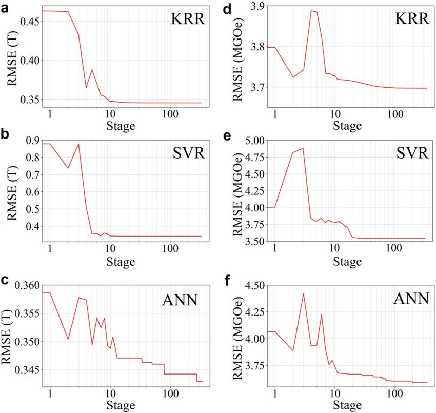
www.nature.com/scientificreports/

                                            Figure 2.  Results of micromagnetic simulations. Scatter plots display the dependence of aint, Dgrain, and
                                            σθ on (a) coercivity and (b) BHmax with the Pearson correlation coefficient (ρ) of each plot indicated in the
                                            inset. The expressions for polynomial fits are µ0 Hc (T) = −2.101σθ3 + 5.940σθ2 − 6.942σθ + 4.875 and
                                            BHmax (MGOe) = −66.05σθ3 − 99.98σθ2 + 1.381σθ + 64.78. In order to investigate the non-linear correlations
                                            between those variables on both coercivity and BHmax, scatter plots are displayed with the x-axis indicating aint,
                                            the y-axis indicating σθ, and the color of dots indicating (c) coercivity and (d) BHmax. Also, violin plots for (e)
                                            z-scores of aint, Dgrain, and σθ, and (f) coercivity and BHmax are displayed where the outer curves represent the
                                            kernel density with the middle line indicating the median. Vertical lines extend and end up in the whiskers,
                                            which indicate the lowest and the highest non-outlier data.

          Scientific Reports |   (2021) 11:3792 |                https://doi.org/10.1038/s41598-021-83315-9                                                       4

Vol:.(1234567890)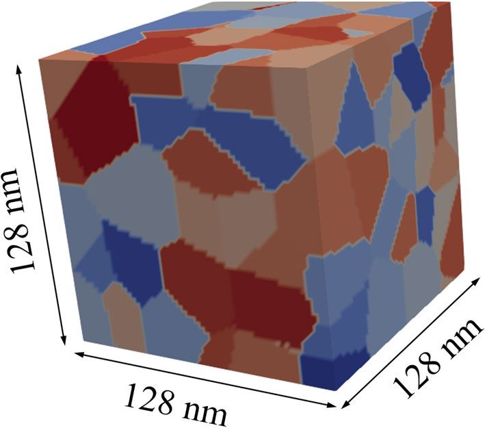
www.nature.com/scientificreports/
Figure 3. Profiles of RMSE by VFSA coupled with different ML models. The profile of the RMSE between the
predicted and actual values of coercivity as optimized with the (a) KRR, (b) SVR, and (c) ANN models and
of BHmax as optimized with the (d) KRR, (e) SVR, and (f) ANN models indicate two phases: a high degree of
randomness at the initial stages (1–10) and a gradual minimization at the latter stages (10–100).
Model Hyper-parameters Values for coercivity prediction Values for BHmax prediction
α 1.7342 × 10⁻⁶ 2.6823 × 10⁻¹⁰
KRR
γ 7.7116 × 10 –4
7.3982 × 10⁻³
C 43.598 1.6339
SVR γ 0.27035 0.11523
ε 3.3378 × 10⁻² 1.5773
α 5.4887 × 10⁻³ 0.17893
ANN
Activation function type tanh ReLU
Table 1. Hyper-parameter values obtained by VFSA for three ML models for the prediction for both
coercivity and BHmax.
tary Information Sect. II. The reasonable agreement between the ML prediction and micromagnetics calculation
shows the predictive ability of the models even when using only a handful of microstructural features.
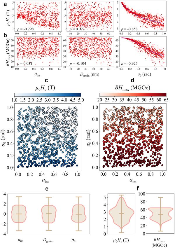
Residual analysis. Furthermore, in the prediction results for BHmax, we identified seven outliers (blue
translucent dots in Fig. 4b) that had the largest biases between the prediction and real data value. We found out
that, by the presence of these outliers, the normality of residuals for the ML models predicting BHmax was broken.
In Fig. 5a, b, quantile–quantile (Q–Q) plots for the residuals between the predictions and real datasets are dis-
played. Note that an unbiased model would have a normal distribution of residuals and thus a linear Q–Q plot.
Then, we again normalized the residuals in order to compare them with a normal distribution and plotted them
against the theoretical quantiles of the normal distribution. In terms of the Pearson correlation coefficient, the
Q–Q plots were almost linear (ρ ≈ 1) in the cases of the coercivity predictions of the three ML models, whereas
they were non-linear (ρ ≪ 1) in the cases of BHmax. Nonetheless, we found that over-fitting, as indicated by four-
fold cross-validation, was not detected, as shown in Supplementary Information Sect. III.
Discussion
In order to overview the dependences of coercivity and BHmax with respect to the input parameters, we predicted
those values from 42,875 artificially generated data as shown in Fig. 6a,b. The predictions were obtained from
ensemble averages of coercivity and BHmax from the KRR, SVR, and ANN models, as shown in Supplementary
Information Sect. IV. The three-dimensional plots revealed the dominance of the three different input param-
eters (i.e., the misalignment of easy axes of grains, inter-grain exchange coupling, and grain size) in determining
coercivity and BHmax. Note that for sufficiently large misalignments of the easy axes, the dependences of coer-
civity and BHmax on inter-grain exchange coupling are opposite to each other. The weak inter-grain exchange
Scientific Reports | (2021) 11:3792 | https://doi.org/10.1038/s41598-021-83315-9 5
Vol.:(0123456789)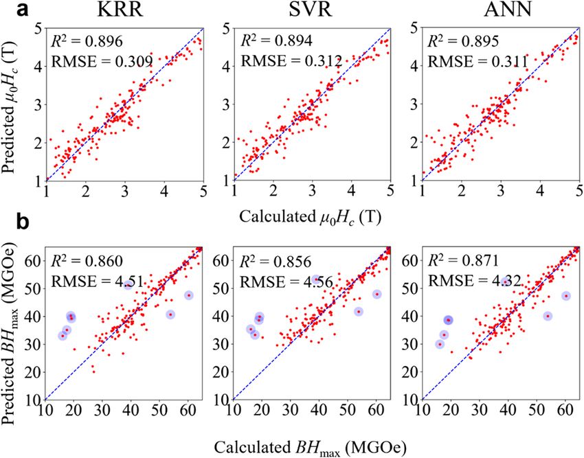
www.nature.com/scientificreports/
Figure 4. Prediction of final ML models optimized by VFSA with coefficient of determination (R2) and RMSE
indicated as insets. (a) Prediction of coercivity by KRR, SVR, and ANN models. (b) Prediction of BHmax
by KRR, SVR, and ANN models. The units of RMSE in (a) and (b) are T and MGOe, respectively. The blue
translucent dots in (b) indicate the seven outliers with the largest residuals.
Figure 5. Q–Q plots for z-scores of residuals between predicted and actual values with Pearson correlation
coefficient of each plot indicated in insets. (a) Q–Q plots obtained from prediction of coercivity by KRR, SVR,
and ANN models. (b) Q–Q plots obtained from prediction of BHmax by KRR, SVR, and ANN models. The gray
lines in each graph are the trend lines to which the ideal Q–Q plot in each case should correspond.
coupling slightly lowers remanent magnetization and the overall coercivity, but also prevents the propagation
of the reversed domains into the neighboring grains, which makes the nucleation-controlled magnetization
reversal process more p referable33. In Fig. 6c are shown two different demagnetization curves representing weak
and strong inter-grain exchange coupling (aint = 0.10 vs. 0.78) for sufficiently large misalignments (σθ = 0.942
and 0.929).
A few data were detected as outliers, particularly in the BHmax prediction, as marked with the blue dots in
Fig. 4b, because there were unusual features involved in their corresponding model geometry. As explained
in Ref.13, the weakest grains in a polycrystalline hard-magnetic cuboid are placed at the edges of the upside or
downside plane of cuboids because demagnetization fields are concentrated there. That is, whether a grain is weak
or not is largely determined by its geometrical position inside of cuboids. As the number of grains per cuboid
decreases, both the average size of grains and the surface-to-volume ratio of each grain increase. Thus, the por-
tion of weakest grains, which cover the surfaces, is higher in a coarse-grained cuboid than in a fine-grained one.
Figure 7a demonstrates in the case of the ANN model, where the seven outliers were all found in coarse-grained
cuboids, or cuboids with large Dgrain or a small number of grains. Also, Fig. 7b displays the cuboid models for
each of the seven outliers, where large and coarse grains occupy the surfaces of the cuboid. We believe that over-
or under-estimation of predicted values of BHmax occurred in those specific coarse-grained cuboids, because
Scientific Reports | (2021) 11:3792 | https://doi.org/10.1038/s41598-021-83315-9 6
Vol:.(1234567890)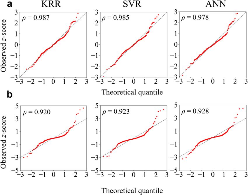
www.nature.com/scientificreports/
Figure 6. Dependences of coercivity and BHmax on input parameters. Ensemble of (a) coercivities and (b)
BHmax values predicted from KRR, SVR and ANN models. The annotated numbers on the contour planes
denote the values of coercivity and BHmax in the units of T and MGOe, respectively. The contour plots were
created with ParaView. (c) Demagnetization curves for different sets of indicated aint and σθ values.
the ML models were unable to consider the irregular changes of BHmax in them. Regardless, further studies are
needed for a more qualitative description.
We expect that GPU-based micromagnetic simulations and optimization of ML models by metaheuristics
such as simulated annealing, genetic algorithm, and tabu search would facilitate the optimal design and/or pro-
cess of microstructures of hard magnets with the aid of advanced fabrication technologies. For example, minutely
increased grain boundary width and external alignment field leads to substantial decoupling between g rains4
and grain a lignment31. Furthermore, in the past, ML models poorly optimized by brute-force techniques such as
grid search and random search were adopted in a variety of studies21–23. The metaheuristics we employed in this
study, VFSA, are based on a concept easy to understand and employ. As such, our work can be said to provide a
cornerstone for future ML studies employing VFSA.
In summary, in order to predict the coercivity and BHmax of NdFeB magnets by ML and search for appro-
priate models, first we constructed, by micromagnetic simulations, a dataset of the correlation between the
microstructural features of granular NdFeB magnets (average grain size, misalignment of easy axes, inter-grain
decoupling) and their macroscopic properties (coercivity and BHmax). We revealed that ML models combined
with VFSA and an adaptive cooling schedule well predict, according to a variety of microstructural param-
eters, the coercivity as well as BHmax of NdFeB magnets. Coercivity had little relationships with respect to Dgrain
but had a non-linear type of relationship with respect to both aint and σθ. This unusual behavior contradicts
the phenomenological theory whereby coercivities are linearly dependent on grain sizes on ~ μm scales. We
believe that this partly results from the averaged-out irregular shape factors. On the other hand, BHmax had a
non-linear type of relationship with respect only to misalignment of easy axes. These results, though obtained
under the specific conditions of grain sizes on ~ nm scales, are invaluable in that only a few researchers31 have
experimentally attempted to correlate BHmax with microstructural factors. Based on the present application of
the VFSA method combined with the KRR, SVR, and ANN models, it was determined that all of the models
provided similar performances in predicting both coercivity and BHmax. Especially, for the prediction of BHmax,
we detected seven outliers (i.e. over- or under-estimation of BHmax) due to which the quality of the used models
was deteriorated. These outliers had appeared owing to too-large sizes of grains covering the top and/or bottom
of the cuboid geometry, leading to irregular values of BHmax that the models could not consider. Further, the
elimination of those outliers resulted in much better performance in the prediction of BHmax, yielding better-
quality ML models. The ML combined with micromagnetic simulation study provided a robust framework for
the design of optimal microstructures of high-performance NdFeB magnets without any need for painstaking
micromagnetic simulations and/or delicate experiments. Furthermore, our results demonstrated the potential of
ML for the design of optimal microstructures of NdFeB magnets, notwithstanding the fact that the underlying
microstructure-property relationships remain unclear.
Scientific Reports | (2021) 11:3792 | https://doi.org/10.1038/s41598-021-83315-9 7
Vol.:(0123456789)www.nature.com/scientificreports/
Figure 7. Origin of seven outliers. (a) Residuals between predicted and actual values of BHmax against the
number of grains and Dgrain as obtained using ANN model. The seven outliers with residuals larger than 13
MGOe are indicated by the blue translucent dots. (b) Model cuboids for seven outliers with grains indicated by
different colors. The model cuboids were visualized with ParaView.
Methods
Micromagnetic simulations. For reliable learning of training data, a large number of datasets including
demagnetization and B–H curves should be prepared. For this purpose, we employed a GPU-accelerated micro-
magnetics package, Mumax3, which incorporates the Landau-Lifshitz-Gilbert (LLG) equation. The package,
based on a finite difference method, calculates the demagnetization curves for a single polycrystalline NdFeB
system composed of 64 × 64 × 64 cells. We used the ‘ext_make3dgrain’ function incorporated into Mumax3
in order to generate the polycrystalline granular structures. Since this function is based on three-dimensional
Voronoi tessellation with randomly chosen crystal seeds, the distribution of grain sizes in our multi-grain model
was totally random. We generated all of the necessary codes responsible for 1000 polycrystalline NdFeB models,
and executed each code in order to obtain the demagnetization curve and the corresponding B–H curve, from
which coercivity and BHmax were extracted, respectively.
Each simulation model had 5 − 256 grains with average grain sizes (Dgrain) ranging from 8 to 64 nm. Further,
in order to examine the effect of misalignment of individual grains’ uniaxial magnetic anisotropy orientation on
coercivity and BHmax, we assumed Gaussian distributions34 with standard deviations of σθ (rad) ∈ [0, 1] for the
angle between the grains’ easy axis and z-axis, θ. Here, the bound of 1 rad corresponds to the average alignment
of easy axes when the perpendicular aligning field is 0.05 T 31. We utilized the following magnetic parameters
corresponding to N dFeB 35: saturation magnetic polarization JS = 1.61 T , exchange stiffness constant
Aex = 12.5 pJ/m , reduced parameter aint = Aint /Aex ∈ [0, 1] where Aint is the inter-grain exchange stiffness
constant, and first-order magnetic anisotropy constant K1 = 4.5 MJ/m3. The size of mesh
discretizing the cuboid
model was set to 2 nm, which is close to the exchange length of NdFeB material, Aex K1 = 1.7 nm.
Details of ML models. The microstructural features used to train the models were of three types: reduced
inter-grain exchange stiffness (aint), average grain size (Dgrain), and degree of misalignment of easy axes (σθ).
In the present work, all of the optimization problems were solved by scikit-learn implementation. The hyper-
Scientific Reports | (2021) 11:3792 | https://doi.org/10.1038/s41598-021-83315-9 8
Vol:.(1234567890)www.nature.com/scientificreports/
parameters of each supervised ML models were optimized by the VFSA algorithm36,37. The types and details of
the ML models employed in this work are as follows.
Kernel ridge regression. Kernel ridge regression (KRR) is a classic approach that constrains model parameter
magnitudes. It limits the sum
of squared errors
by
imposing an L2-norm, which is the sum of squares of weights
w. Given a training dataset x1 , y1 , · · · , xn , yn , this is equivalent to minimizing the objective function38
n
1 1
(yi − w T φ(xi ))2 + α�w�2
2 2
i=1
where φ : Rn → R is a kernel function that maps xi ∈ Rn to the feature space. In this work, a radial basis func-
tion φ(xi ) = exp(−γ �xi �2 ) was employed as the kernel function. The second term is the regularization term in
which α acts as a weight that balances minimization of the sum of squared errors and limits the complexity of the
model. In general, the larger the value of α, the lower the magnitude of parameters and thus of the complexity
of the model38. There were two hyper-parameters of KRR model to be optimized: the coefficient of the kernel
function γ and the regularization parameter α.
Support vector regression. Support vector regression (SVR) is a non-linear regression analysis based on sup-
port vector machine, which is again rooted in statistical learning or Vapnik–Chervonenkis t heory26,27. The loss
functions for ordinary regression analysis are sums of squares of error, whereas that of SVR is an ε-insensitive
loss function of linear, quadratic, or Huber type. In ε-SVR, the goal is to find a function f(x) that has at most ε
deviation from the actually obtained targets yi for all training data, and at the same time is as flat as possible, i.e.
with as small weights as possible.
Suppose we are given a training dataset x1 , y1 , · · · , xn , yn , where xi is a vector of independent variables
and yi is a corresponding scalar-dependent variable. Then, the function in the feature space is approximated by
f (x) = w T φ(x) + b, where w defines the weight vector, b is a bias parameter, and φ(x) is a kernel function that
maps x to the feature space. In the present work, a radial basis function φ(xi ) = exp(−γ �xi �2 ) was employed as
the kernel. The loss function to be minimized is described by
n
1
�w�2 + C Eε (yi , f (xi ))
2
i=1
where C is the regularization parameter and Eε (y, f (xi )) is the ε-insensitive loss function. There were three hyper-
parameters to be optimized: C, ε, and γ.
Artificial neural network. For artificial neural network (ANN) regression28, we used the MLPRegressor module
implemented in the scikit-learn package. The L2 regularization parameter, α, and the type of activation functions
(allowed to shift between a hyperbolic tangent function (tanh), a sigmoid function (logistic), and a rectified
linear unit function (ReLU)) employed in this method were two hyper-parameters to be optimized. However,
the optimization method was restricted to the limited-memory Broyden–Fletcher–Goldfarb–Shanno (L-BFGS)
method, as were the number of hidden layers and neurons, to 1 and 100, respectively, for simplicity. In addition,
we used the mean squared error with L2-penalty as the loss function.
Simulated annealing. We employed the VFSA algorithm proposed by Szu and Hartley39 and improved by
Ingber40. Also, we adopted an adaptive cooling schedule, according to which the temperature at the j th stage is
calculated by
Tj
Tj+1 = ,
1 + exp[−(f (xcand ) − f (xcurr ))/T0 ]
where f (x) is the objective function to optimize, xcurr is the current solution, xcand is the candidate solution, and
T0 is the initial temperature. This kind of cooling scheme is based on idea that keeps the temperature unchanged
when the value of the objective function for the candidate solution is far from that for the global optimum and
that halves the temperature when the solution is updated ( f (xcurr ) = f (xcand )). The RMSE between the actual
datasets as calculated from micromagnetic simulation and those predicted from ML model was used as the objec-
tive function in this scheme. Further, the initial temperature was set such that the acceptance probability at the
initial stage is 0.7, in order to avoid redundant initial stages with a high degree of r andomness41, and the final
temperature was set to be sufficiently low, at 10−100. At each temperature, the neighborhoods of the candidate
solution were searched 100 times.
Received: 24 November 2020; Accepted: 2 February 2021
References
1. Sagawa, M., Fujimura, S., Togawa, N., Yamamoto, H. & Matsuura, Y. New material for permanent magnets on a base of Nd and Fe
(invited). J. Appl. Phys. 55, 2083 (1984).
Scientific Reports | (2021) 11:3792 | https://doi.org/10.1038/s41598-021-83315-9 9
Vol.:(0123456789)www.nature.com/scientificreports/
2. Gutfleisch, O. et al. Magnetic materials and devices for the 21st century: Stronger, lighter, and more energy efficient. Adv. Mater.
23, 821–842 (2011).
3. Herbst, J. F. R 2F14B materials: Intrinsic properties and technological aspects. Rev. Mod. Phys. 63, 819 (1991).
4. Sasaki, T. T. et al. Formation of non-ferromagnetic grain boundary phase in a Ga-doped Nd-rich Nd–Fe–B sintered magnet. Scr.
Mater. 113, 218–221 (2016).
5. Bance, S. et al. Grain-size dependent demagnetizing factors in permanent magnets. J. Appl. Phys. 116, 233903 (2014).
6. Kronmüller H. & Fähnle, M. Coercivity of modern magnetic materials in Micromagnetism and the Microstructure of Ferromagnetic
Solids 90–147 (Cambridge University Press, 2003).
7. Kim, S.-K., Hwang, S. & Lee, J.-H. Effect of misalignments of individual grains’ easy axis on magnetization-reversal process in
granular NdFeB magnets: A finite-element micromagnetic simulation study. J. Magn. Magn. Mater. 486, 165257 (2019).
8. Pilania, G., Wang, C., Jiang, X., Rajasekaran, S. & Ramprasad, R. Accelerating materials property predictions using machine learn-
ing. Sci. Rep. 3, 2810 (2013).
9. Iwasaki, Y. et al. Machine-learning guided discovery of a new thermoelectric material. Sci. Rep. 9, 2751 (2019).
10. Butler, K. T., Frost, J. M., Skelton, J. M., Svanea, K. L. & Walsh, A. Computational materials design of crystalline solids. Chem. Soc.
Rev. 45, 6138–6146 (2016).
11. Chandrasekaran, A., Kamal, D., Batra, R., Kim, C., Chen, L. & Ramprasad, R. Solving the electronic structure problem with machine
learning. npj Comput. Mater. 5, 22 (2019).
12. Möller, J. J., Körner, W., Krugel, G., Urban, D. F. & Elsässer, C. Compositional optimization of hard-magnetic phases with machine-
learning models. Acta Mater. 153, 53–61 (2018).
13. Exl, L. et al. Magnetic microstructure machine learning analysis. J. Phys. Mater. 2, 014001 (2018).
14. Gusenbauer, M. et al. Extracting local nucleation fields in permanent magnets using machine learning. npj Comput. Mater. 6, 89
(2020).
15. Cheng, W. Magnetic properties prediction of NdFeB magnets by using support vector regression. Mod. Phys. Lett. B 28, 1450177
(2014).
16. Stoner, E. C. & Wohlfarth, E. P. A mechanism of magnetic hysteresis in heterogeneous alloys. Philos. Trans. R. Soc. A240, 599–642
(1948).
17. Skomski, R., Schubert, E., Enders, A. & Sellmyer, D. J. Kondorski reversal in magnetic nanowires. J. Appl. Phys. 115, 17D137 (2014).
18. Matsuura, Y., Hoshijima, J. & Ishii, R. Relation between Nd2Fe14B grain alignment and coercive force decrease ratio in NdFeB
sintered magnets. J. Magn. Magn. Mater. 336, 88–92 (2013).
19. Bance, S. et al. Influence of defect thickness on the angular dependence of coercivity in rare-earth permanent magnets. Appl. Phys.
Lett. 104, 182408 (2014).
20. Li, J. et al. Angular dependence and thermal stability of coercivity of Nd-rich Ga-doped Nd–Fe–B sintered magnet. Acta Mater.
187, 66–72 (2020).
21. Schulz, M.-A. et al. Different scaling of linear models and deep learning in UKBiobank brain images versus machine-learning
datasets. Nat. Commun. 11, 4238 (2020).
22. Yoo, T. K. et al. Adopting machine learning to automatically identify candidate patients for corneal refractive surgery. npj Digit.
Med. 2, 59 (2019).
23. Leger, S. et al. A comparative study of machine learning methods for time-to-event survival data for radiomics risk modelling. Sci.
Rep. 7, 13206 (2017).
24. Lombardi, A. M. Estimation of the parameters of ETAS models by simulated annealing. Sci. Rep. 5, 8417 (2015).
25. Zhao, Y. et al. Broadband diffusion metasurface based on a single anisotropic element and optimized by the simulated annealing
algorithm. Sci. Rep. 6, 23896 (2016).
26. Smola, A. J. & Schölkopf, B. A tutorial on support vector regression. Stat. Comput. 14, 199–222 (2004).
27. Awad, M. & Khanna, R. Support vector regression. in Efficient Learning Machines: Theories, Concepts, and Applications for Engineers
and System Designers 67–80 (Apress, 2015).
28. Schmidhuber, J. Deep learning in neural networks: An overview. Neural Netw. 61, 85–117 (2015).
29. Han, G. B. et al. Effect of exchange–coupling interaction on the effective anisotropy in nanocrystalline Nd2Fe14B material. J. Magn.
Magn. Mater. 281, 6–10 (2004).
30. Yang, H., Liu, M., Lin, Y. & Yang, Y. Simultaneous enhancements of remanence and (BH)max in BaFe12O19/CoFe2O4 nanocomposite
powders. J. Alloys Compd. 631, 335–339 (2015).
31. Gao, R. W., Zhang, D. H., Li, H. & Zhang, J. C. Effects of the degree of grain alignment on the hard magnetic properties of sintered
NdFeB magnets. Appl. Phys. A 67, 353–356 (1998).
32. Zheng, A. & Casari, A. Fancy tricks with simple numbers. in Feature Engineering for Machine Learning: Principles and Techniques
for Data Scientists (Ed. Roumeliotis, R. & Bleiel, J.) 5–39 (O’Reilly, 2018).
33. Lee, J.-H., Choe, J., Hwang, S. & Kim, S.-K. Magnetization reversal mechanism and coercivity enhancement in three-dimensional
granular Nd-Fe-B magnets studied by micromagnetic simulations. J. Appl. Phys. 122, 073901 (2017).
34. Tenaud, P., Chamberod, A. & Vanoni, F. Texture in Nd–Fe–B magnets analysed on the basis of the determination of Nd2Fe14B
single crystals easy growth axis. Solid State Commun. 63, 303–305 (1987).
35. Sagawa, M., Fujimura, S., Yamamoto, H., Matsuura, Y. & Hirosawa, S. Magnetic properties of rare-earth-iron-boron permanent
magnet materials. J. Appl. Phys. 57, 4094 (1985).
36. Kirkpatrick, S., Gelatt, C. D. Jr. & Vecchi, M. P. Optimization by simulated annealing. Science 220, 671–680 (1983).
37. Jansen, T. Simulated annealing. in Theory of Randomized Search Heuristics (Ed. Auger A. & Doerr, B) 171–195 (World Scientific,
2011).
38. Lever, J., Krzywinski, M. & Altman, N. Regularization. Nat. Methods 13, 803–804 (2016).
39. Szu, H. & Hartley, R. Fast simulated annealing. Phys. Lett. A 122, 157–162 (1987).
40. Ingber, L. Very fast simulated re-annealing. Math. Comput. Model. 12, 967–973 (1989).
41. Aarts, E., Korst, J. & van Laarhoven, P. Simulated annealing. in Local Search in Combinatorial Optimization (Ed. Aarts, E. & Lenstra,
J. K.) 91–120 (Wiley, 1997).
Acknowledgements
This research was supported by the National R&D Program through the National Research Foundation of Korea
(NRF) funded by the Ministry of Science and ICT (grant No. NRF-2020M3H4A3105640), by the Korea Institute
of Energy Research (Expanding Platform Technology for Energy R&D Innovation, C0-2435), and by the BK21
PLUS SNU Materials Education/Research Division for Creative Global Leaders. The Institute of Engineering
Research at Seoul National University provided additional research facilities for this work.
Scientific Reports | (2021) 11:3792 | https://doi.org/10.1038/s41598-021-83315-9 10
Vol:.(1234567890)www.nature.com/scientificreports/
Author contributions
H.-K. P. and S.-K. K. conceived the main idea and planned the micromagnetic simulations. H.-K. P. performed
the micromagnetic simulations and analyzed the data along with J. L. H.-K. P. wrote the manuscript with the
help of J.-H. L., J. L., and S.-K. K.
Competing interests
The authors declare no competing interests.
Additional information
Supplementary Information The online version contains supplementary material available at https://doi.
org/10.1038/s41598-021-83315-9.
Correspondence and requests for materials should be addressed to J.L. or S.-K.K.
Reprints and permissions information is available at www.nature.com/reprints.
Publisher’s note Springer Nature remains neutral with regard to jurisdictional claims in published maps and
institutional affiliations.
Open Access This article is licensed under a Creative Commons Attribution 4.0 International
License, which permits use, sharing, adaptation, distribution and reproduction in any medium or
format, as long as you give appropriate credit to the original author(s) and the source, provide a link to the
Creative Commons licence, and indicate if changes were made. The images or other third party material in this
article are included in the article’s Creative Commons licence, unless indicated otherwise in a credit line to the
material. If material is not included in the article’s Creative Commons licence and your intended use is not
permitted by statutory regulation or exceeds the permitted use, you will need to obtain permission directly from
the copyright holder. To view a copy of this licence, visit http://creativecommons.org/licenses/by/4.0/.
© The Author(s) 2021
Scientific Reports | (2021) 11:3792 | https://doi.org/10.1038/s41598-021-83315-9 11
Vol.:(0123456789)You can also read