Lost! Leveraging the Crowd for Probabilistic Visual Self-Localization
←
→
Page content transcription
If your browser does not render page correctly, please read the page content below
Lost! Leveraging the Crowd for Probabilistic Visual Self-Localization

           Marcus A. Brubaker                            Andreas Geiger                         Raquel Urtasun
              TTI Chicago                              KIT & MPI Tübingen                       TTI Chicago
      mbrubake@cs.toronto.edu                          geiger@kit.edu                        rurtasun@ttic.edu

                        Abstract

    In this paper we propose an affordable solution to self-
localization, which utilizes visual odometry and road maps
as the only inputs. To this end, we present a probabilis-
tic model as well as an efficient approximate inference al-
gorithm, which is able to utilize distributed computation
to meet the real-time requirements of autonomous systems.
Because of the probabilistic nature of the model we are
able to cope with uncertainty due to noisy visual odometry
and inherent ambiguities in the map (e.g., in a Manhattan           Figure 1. Visual Self-Localization: We demonstrate localizing
world). By exploiting freely available, community devel-            a vehicle with an average accuracy of 3.1m within a map of ∼
                                                                    2, 150km of road using only visual odometry measurements and
oped maps and visual odometry measurements, we are able
                                                                    freely available maps. In this case, localization took less than 21
to localize a vehicle up to 3m after only a few seconds of
                                                                    seconds. Grid lines are every 2km.
driving on maps which contain more than 2,150km of driv-
able roads.                                                         taining an up-to-date world representations will be feasi-
                                                                    ble given the computation, memory and communication re-
                                                                    quirements. Furthermore, these solutions are far from af-
1. Introduction                                                     fordable as every corner of the world needs to be visited
    Self-localization is key for building autonomous systems        and updated constantly. Finally, privacy and security issues
that are able to help humans in everyday tasks. Despite             need to be considered as the recording and storage of such
decades of research, it is still an exciting open problem. In       data is illegal in some countries.
this paper we are interested in building affordable and ro-             In contrast to the above mentioned approaches, here we
bust solutions to self-localization for the autonomous driv-        tackle the problem of self-localization in places that we
ing scenario. Currently, the leading technology in this set-        have never seen before. We take our inspiration from hu-
ting is GPS. While being a fantastic aid for human driv-            mans, which excel in this task while having access to only
ing, it has some important limitations in the context of au-        a rough cartographic description of the environment. We
tonomous systems. Notably, the GPS signal is not always             propose to leverage the crowd, and exploit the development
available, and its localization can become imprecise (e.g.,         of OpenStreetMap (OSM), a free community-driven map,
in the presence of skyscrapers, tunnels or jammed signals).         for the task of vision-based localization. The OSM maps
While this might still be viable for human driving, conse-          are detailed and freely available, making this an inexpen-
quences can be catastrophic for self-driving cars.                  sive solution. Moreover, they are more frequently updated
    To provide alternatives to GPS localization, place recog-       than their commercial counterparts. Towards this goal, we
nition approaches have been developed. They assume that             derive a probabilistic map localization approach that uses
image or depth features from anywhere around the globe              visual odometry estimates and OSM data as the only inputs.
can be stored in a database, and cast the localization prob-        We demonstrate the effectiveness of our approach on a va-
lem as a retrieval task. Both 3D point clouds [5, 7, 10, 20]        riety of challenging scenarios making use of the recently
and visual features [2, 3, 11, 15, 16, 24] have been lever-         released KITTI visual odometry benchmark [8]. As our ex-
aged to solve this problem. In combination with GPS, im-            periments show, we are able to localize ourselves after only
pressive results have been demonstrated (e.g., the Google           a few seconds of driving with an accuracy of 3 meters on a
self-driving car). However, it remains unclear if main-             18km2 map containing 2, 150km of drivable roads.

                                                                1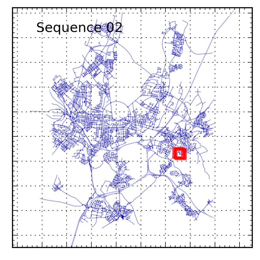
3. Visual Localization
We propose to use one or two roof-mounted cameras to
self-localize a driving vehicle. The only other information
we have is a map of the environment in which the vehicle is
driving. This map contains streets as line segments as well
as intersection points. We exploit visual odometry in or-
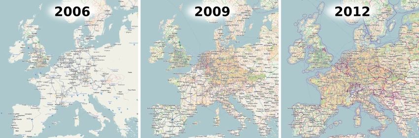
Figure 2. Evolution of OpenStreetMap coverage from 2006- der to obtain the trajectory of the vehicle. As this trajectory
2012: As of 2012, over 3 billion GPS track points have been added is too noisy for direct shape matching, here we propose a
and 1.6 billion nodes / 150 million line segments have been created probabilistic approach to self-localization that employs vi-
by the community. Here we use OSM maps and visual odometry sual odometry measurements in order to determine the in-
estimates as the only inputs for localizing within the map. stantaneous position and orientation of the vehicle in a given
map. Towards this goal, we first define a graph-based rep-
2. Related Work resentation of the map as well as a probabilistic model of
Early approaches for map localization [5, 7, 10, 20] how a vehicle can traverse the graph. For inference, we de-
make use of Monte Carlo methods and the Markov assump- rive a filtering algorithm, which exploits the structure of the
tion to maintain a sample-based posterior representation of graph using Mixtures of Gaussians. In order to keep running
the agent’s pose. However, they only operate locally with- times reasonable, we further propose techniques for limiting
out providing any global (geographic) positioning informa- the complexity of the mixture models which includes an al-
tion and thus can not be applied to the problem we consider gorithm for simplifying the Gaussian Mixture models. We
here. Furthermore, they are typically restricted to small- start our discussion by presenting the employed map infor-
scale environments and low-noise laser-scan observations. mation, followed by our probabilistic model.
At a larger scale, place recognition methods localize
3.1. The OpenStreetMap Project
[2, 11, 16, 24] or categorize [22, 23, 27] an image, given a
database of geo-referenced images or video streams [3, 15]. Following the spirit of Wikipedia, Steve Coast launched
While processing single landmarks is clearly feasible, cre- the OpenStreetMap (OSM) project in 2004 with the goal
ating an up-to-date “world database” seems impractical due of creating a free editable map of the world. So far, more
to computational and memory requirements. In contrast, the than 800,0002 users around the globe have contributed by
maps used by our localization approach require only a few supplying tracks from portable GPS devices, labeling ob-
gigabytes for storing the whole planet earth1 . jects using aerial imagery or providing local information.
Relative motion estimates can be obtained using visual Fig. 2 illustrates the tremendous growth of OSM over the
odometry [19], which refers to generating motion estimates last years. Compared to commercial products like Google
from visual input alone. While current implementations Maps, the provided data is more up-to-date, often includes
[1, 9, 14] demonstrate impressive performance [8], their more details (e.g., street types, traffic lights, postboxes,
incremental characteristics inevitably leads to large drift at trees, shops, power lines) and – most importantly – can be
long distances. Methods for Simultaneous Localization And freely downloaded and used under the Open Database Li-
Mapping (SLAM) [18, 25, 6] are able to reduce this drift by cense. We extracted all crossings and drivable roads (rep-
modelling the map using landmarks and jointly optimizing resented as piece-wise linear segments) connecting them.
over poses and landmarks. Limitations in terms of speed For each street we additionally extract its type (i.e., high-
and map size have been partially overcome, for example way or rural) and the direction of traffic. By splitting each
by efficient optimization strategies using incremental sparse bi-directional street into two one-way streets and ’smooth-
matrix factorization [13] or the use of relative representa- ing’ intersections using circular arcs, we obtain a lane-based
tions [17]. Furthermore, recent progress in loop-closure de- map representation, on which we define the vehicle state.
tection [4, 21, 26] has led to improved maps by constrain-
ing the problem at places which have been visited multiple 3.2. Lane-based Map Representation
times. However, SLAM methods can only localize them- We assume that the map data is represented by a directed
selves in maps that have been previously created with a sim- graph where nodes represent street segments and edges de-
ilar sensor setup, hence strongly limiting their application fine the connectivity of the roads. Roads which dead-end or
at larger scales. In contrast, the proposed approach enables run off the edge of the map are connected to a “sink” node.
geographic localization and relies only on freely available As mentioned above, we convert all street segments to one-
map information (i.e., OpenStreetMap). To our knowledge, way streets. An example of a map and corresponding graph
ours is the first approach in this domain. representation is shown in Fig. 3 (left). Each street segment
1 http://wiki.openstreetmap.org/wiki/planet.osm 2 http://wiki.openstreetmap.org/wiki/stats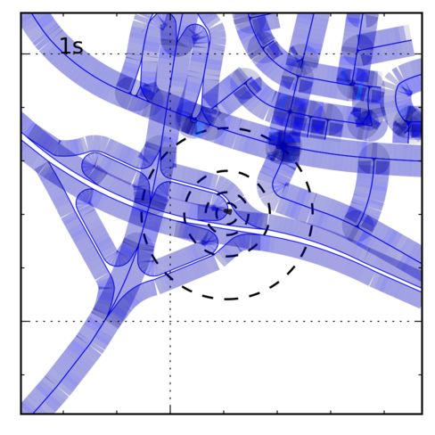
models to be both simple and effective. Because the com-
SINK
6
d
θ �
� p1 ponents of st are relative to the current street, ut , when
1 5 ut 6= ut−1 the state transition model must be adjusted so
that st becomes relative to ut . Both dt and dˆt−1 must have
6 5
r ψ0
1 4 ψ1 `ut−1 subtracted, and θ̂t−1 needs to be updated so that θ̂t−1
2 4 β
relative to ut has the same global heading as θt−1 relative
Origin p0 c
3 2 3
to ut−1 . The above model can then be expressed as
Figure 3. Map Graph: (left) A simple map and its corresponding
2 −1 0 0
graph representation. Street Segment: (right) Each street segment 1 0 0 0
has a start and end position p0 and p1 , a length `, an initial heading Aut ,ut−1 = 0
(3)
of the street segment β and a curvature parameter α = ψ1 −ψ 0
. For
0 γut 0
`
arc segments c is the circle center, r is the radius and ψ0 and ψ1 0 αut−1 − αut 1 0
(
are the start and end angles of the arc. For linear segments, α = 0. −(`ut−1 , `ut−1 , 0, θut ,ut−1 )T ut 6= ut−1
but ,ut−1 = (4)
(0, 0, 0, 0)T ut = ut−1
is either a linear or a circular arc segment. The parame- where θut ,ut−1 = βut − (βut−1 + αut `ut−1 ) is the angle
ters of the street segment geometry are described in Fig. 3 between the end of ut and the beginning of ut−1 .
(right). We define the position and orientation of a vehicle The street transition probability p(ut |xt−1 ) defines the
in the map in terms of the street segment u that the vehi- probability of transitioning onto the street ut given the pre-
cle is on, the distance from the origin of that street segment vious state xt−1 . We use the Gaussian transition dynamics
d and the offset of the local street heading θ. The global to define the probability of changing street segments, i.e.,
heading of the vehicle is then θ + β + αd and its position is Z `u +`u
`−d d `−d d
` p0 + ` p1 for a linear segment and c+rd( ` ψ0 + ` ψ1 )
t−1
T p(ut |xt−1 ) = ξut ,ut−1 N (x|aTd st−1 , aTd Σxut−1 ad )dx
for a circular arc segment, with d(θ) = (cos θ, sin θ) . `ut−1
(5)
3.3. State-Space Model where ad = (2, −1, 0, 0),
We define the state of the model at time t to be xt =
1 ut = ut−1
(ut , st ) where st = (dt , dˆt−1 , θt , θ̂t−1 )T and dˆt−1 , θ̂t−1 1
are the distance and angle at the previous time defined rel- ξut ,ut−1 = |N(u j )|
ut ∈ N(ut−1 ) (6)
ative to the current street ut . Visual odometry observations 0 otherwise
at time t, yt , measure the linear and angular displacement
from time t − 1 to time t. We thus model and N(u) is the set of streets to which u connects.
As short segments cannot be jumped over in a single time
p(yt |xt ) = N (yt |Mut st , Σyut ) (1) step, we introduce “leapfrog” edges which allow the vehicle
to move from ut−1 to any ut to which there exists a path in
where Mu = [md , mθ ]T , md = (1, −1, 0, 0)T and mθ = the graph. To handle this properly, we update the entries
(αu , −αu , 1, −1)T . The curvature of the street, αu , is nec- of but ,ut−1 to consider transitioning over a longer path and
essary because the global heading of the vehicle depends ξut ,ut−1 is the product ξ along the path. As the speed of the
on both d and θ. We factorize the state transition distribu- vehicle is assumed to be limited, we need to add edges only
tion p(xt |xt−1 ) = p(ut |xt−1 )p(st |ut , xt−1 ) in terms of the up to a certain distance. Assuming a top speed of around
street transition probability p(ut |xt−1 ), and the state tran- 110km/h and observations every second, we add leapfrog
sition model p(st |ut , xt−1 ). The state transition model is edges for paths of up to 30m.
assumed to be Gauss-Linear, taking the form 3.4. Inference
p(st |ut , xt−1 ) = N (st |Aut ,ut−1 st−1 + but ,ut−1 , Σxut ) Given the above model we wish to compute the filtering
(2) distribution, p(xt |y1:t ). We can write the posterior using
with Σxut the covariance matrix for a given ut which is the product rule as p(xt |y1:t ) = p(st |ut , y1:t )p(ut |y1:t ),
learned from data as discussed in Section 4. We use a where p(ut |y1:t ) is a discrete distribution over streets and
second-order, constant velocity model for the change in d p(st |ut , y1:t ) is a continuous distribution over the position
and a first order autoregressive model, i.e., AR(1), for the and orientation on a given street. We choose to represent
angular offset θ. That is, dt = dt−1 + (dt−1 − dˆt−2 ) plus p(st |ut , y1:t ) using a Mixture of Gaussians, i.e.,
noise, and θt = γut−1 θt−1 plus noise where γut−1 ∈ [0, 1] Nut
X
is the parameter of the AR(1) model which controls the cor- p(st |ut , y1:t ) = πu(i)t N (st |µ(i) (i)
ut , Σut ) (7)
relation between θt and θt−1 . In practice, we found these i=1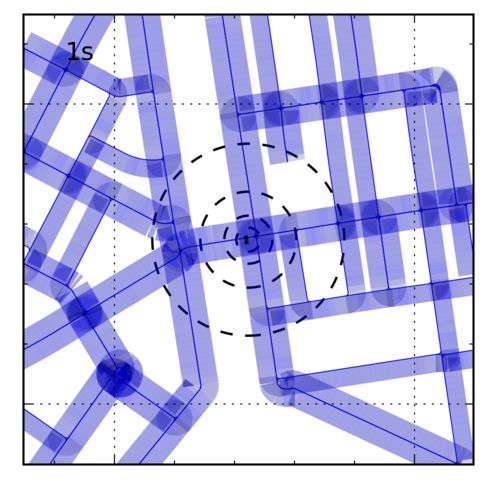
Algorithm 1 Filter
Computation Time Per Frame (s)
25 Monocular 1.0
Monocular
1: Input: Posterior at t−1, {Put−1 , Mt−1 Stereo Stereo
u }, and observation, yt
Position Error (m)
20 0.8 Real-time
2: Initialize mixtures, Mtu ← ∅, for all u 15 0.6
3: for all streets ut−1 do 10 0.4
4: for all streets ut reachable from ut−1 do 5 0.2
0 0.0 -5
5: for k = 1, . . . , |Mt−1
ut−1 | do 10-5 10-4 10-3 10-2 10-1 10 10-4 10-3 10-2 10-1
Simplify Threshold (nats) Simplify Threshold (nats)
6: if p(ut |ut−1 , st−1 ) is approx. constant then
Figure 4. Simplification Threshold: Impact of the simplification
7: Analytically approx. cpred N (µpred , Σpred )
threshold on localization accuracy (left) and computation time
8: else
(right). We use = 10−2 for all other experiments.
9: Sample to compute cpred N (µpred , Σpred )
10: Incorporate yt to compute cupd N (µupd , Σupd ) 65 350
11: Add N (µupd , Σupd ) to Mtui with weight cupd 60 Monocular Monocular
Distance to Localize (m)
300
55 Stereo Stereo
Time to Localize (s)
12: for all streets u do 50 250
45
200
13: Set Put to the sum of the weights of mixture Mtu 40
35 150
14: Normalize the weights of mixture Mtu 30
100
25
15: Normalize Put so that t
P
u Pu = 1. 200.0 0.5 1.0 1.5 2.0 500.0 0.5 1.0 1.5 2.0
Initial Region Size (km) Initial Region Size (km)
16: Return: Posterior at t, {Put , Mtu }
Figure 5. Map Size: Driving time (left) and distance travelled
(right) before localization as a function of the map size.
where Nut is the number of components for the mixture as-
(i) (i) (i) Nut
sociated with ut and Mtut = {πut , µut , Σut }i=1 are the
parameters of the mixture for ut . This is a general and pow- incorporated by multiplying two Gaussian PDFs. This algo-
erful representation but still allows for efficient and accurate rithm can also be parallelized by assigning subsets of streets
inference. Assuming independent observations given the to different threads, a fact which we exploit to achieve real-
states and that the state transitions are first order Markov, time performance. Appendix A gives more details and the
we write the filtering distribution recursively as filtering process is summarized in Algorithm 1.
Z
p(yt |xt )p(xt |xt−1 )
p(xt |y1:t ) = p(xt−1 |y1:t−1 )dxt−1 3.5. Managing Posterior Complexity
p(yt |y1:t−1 )
(8) The previous section provides a basic algorithm to com-
which, after factoring p(xt−1 |y1:t−1 ), gives pute the filtering distributions recursively. Unfortunately, it
X Put−1 Z
is impractical as the complexity of the posterior (i.e., the
p(xt |y1:t ) = p(yt |xt ) p(st |ut , ut−1 , st−1 )
Zt (9) number of mixture components) grows exponentially with
ut−1
time. To alleviate this, we propose three approximations
× p(ut |ut−1 , st−1 )p(st−1 |ut−1 , y1:t−1 )dst−1 which limit the resulting complexity of the posterior. We
where Put−1 = p(ut−1 |y1:t−1 ) and Zt = p(yt |y1:t−1 ). have found these approximations to work well in practice
Substituting in the mixture model form of and to significantly reduce computational costs.
p(st−1 |ut−1 , y1:t−1 ), and the model transition dynamics First, for each pair of connected streets, the modes that
the integrand in the above equation becomes transition from ut−1 to ut are all likely similar. As such, all
N Z of the transitioned modes are replaced with a single com-
X
π (i) p(ut |ut−1 ,st−1 )N (st |Ast−1 + b, Σx ) ponent using moment matching. Second, eventually most
i=1
(10) streets will have negligible probability. Thus, we truncate
the distribution for streets whose probability p(ut |y1:t ) is
× N (st−1 |µ(i) , Σ(i) )dst−1 .
below a threshold and discard their modes. We use a con-
In general, the integral in Eq. (10) is not analytically servative threshold of 10−50 . Finally, the number of compo-
tractable. However, if p(ut |ut−1 , st−1 ) were constant nents in the posterior grows with t. Many of those compo-
the integral could be solved easily. In our model nents will have small weight and be redundant. To prevent
p(ut |ut−1 , st−1 ) is the Gaussian CDF and has a sigmoidal this from happening, we run a mixture model simplification
shape. Because of this, it is approximately constant every- procedure when the number of modes on a street segment
where except near the transition point of the sigmoid. We exceeds a threshold. This procedure removes components
determine whether p(ut |ut−1 , st−1 ) can be considered con- and updates others while keeping the KL divergence below
stant and, if so, use an analytical approximation. Other- a threshold . Details of this approximation can be found
wise, we use a Monte Carlo approximation, drawing sam- in Appendix B, and the effects of varying the maximum al-
ples from N (st−1 |µ(i) , Σ(i) ). Finally the observation yt is lowed KL divergence, , are investigated in the experiments.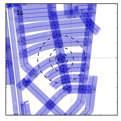
00      01      02       03       04      05      06       07        08       09       10      Average
                   M     15.6m      *     8.1m    18.8m       *     5.6m      *     15.5m     45.2m     5.4m       *       18.4m
                   S     2.1m     3.8m    4.1m    4.8m        *     2.6m      *      1.8m     2.4m      4.2m     3.9m       3.1m
 Position Error
                   G     1.8m     2.5m    2.2m    6.9m        *     2.7m      *      1.5m     2.0m      3.8m     2.5m       2.4m
                   O     0.8m     1.3m    1.0m    2.5m      3.9m    1.3m    1.0m     0.6m     1.1m      1.2m     1.1m      1.44m
                   M      2.0◦      *     1.5◦     2.4◦       *     2.0◦      *      1.3◦     10.3◦     1.6◦       *        3.6◦
 Heading Error     S      1.2◦    2.7◦    1.3◦     1.6◦       *     1.4◦      *      1.9◦      1.2◦     1.3◦     1.3◦       1.3◦
                   G      1.0◦    1.0◦    0.8◦     1.4◦       *     1.2◦      *      1.5◦      1.0◦     0.9◦     1.0◦       1.0◦
Table 1. Sequence Errors: Average position and heading errors for 11 training sequences. “M” and “S” indicate monocular and stereo
odometry, “G” GPS-based odometry and “O” is the oracle error, i.e., the error from projecting the GPS positions onto the map. Chance
performance is 397m. All averages are computed over localized frames (see text) and “*” indicates sequences which did not localize.

4. Experimental Evaluation                                          data to the mean road position of each map.
    To evaluate our approach in realistic situations, we per-           We used the projected GPS data to learn the small num-
formed experiments on the recently released KITTI bench-            ber of model parameters. In particular, the street state evo-
mark for visual odometry [8]. We utilize the 11 training            lution noise covariance Σxu , the angular AR(1) parameter
sequences for quantitative evaluation (where ground truth           γu and the observation noise Σyu were estimated using max-
GPS data is available), and perform qualitative evaluation          imum likelihood. We learn different parameters for high-
on both training and test sequences (see Supplemental Ma-           ways and city/rural roads as the visual odometry performs
terial). This results in 39.2km of driving in total. The visual     significantly worse at higher speeds.
odometry input to our system is computed using LIBVISO2                 The accuracy of position and heading estimates is not
[9], a freely available library for monocular and stereo vi-        well defined until the posterior has converged to a single
sual odometry. To speed up inference, we subsample the              mode. Thus, we only compute accuracy once a sequence
data to a rate of one frame per second. Slower rates were           has been localized. All results are divided into two tempo-
found to suffer from excessive accumulated odometry er-             rally contiguous parts: unlocalized and localized. We define
ror. For illustration purposes, here we extracted mid-size          a sequence to be localized when for at least five seconds
regions of OpenStreetMap data which included the true tra-          there is a single mode in the posterior and the distance to
jectory and the surrounding region. On average, they cover          the ground truth position from that mode is less than 20 me-
an area of 2km2 and contain 47km of drivable roads. It is           ters. Once the criteria for localization is met, all subsequent
important to note that our method also localizes success-           frames are considered localized. Errors in global position
fully on much larger maps, see Fig. 1 for example, which            and heading of the MAP state for localized frames were
covers 18km2 and contains 2,150km of drivable roads. We             computed using the GPS data as ground truth. Sequences
set the simplification threshold to  = 10−2 which is ap-           which did not localize are indicated with a “*” in Table 1.
plied when the number of mixture components for a seg-                  Overall, we are able to estimate the position and head-
ment is greater than one per 10m segment length.                    ing to 3.1m and 1.3◦ using stereo visual odometry. Note
                                                                    that this comes very close to the average oracle error of
Quantitative Evaluation: Quantitative results can be
                                                                    1.44m, the lower bound on the achievable error induced
found in Table 1, with corresponding qualitative results
                                                                    by inaccuracies in the OpenStreetMap data! These results
shown in Fig. 8. Here, “M” and “S” indicate results using
                                                                    also outperform typical consumer grade navigation systems
monocular and stereo visual odometry respectively. In addi-
                                                                    which offer accuracies of around 10 meters at best. Fur-
tion, we computed odometry measurements from the GPS
                                                                    thermore, errors are comparable to those achieved using the
trajectories (entry “G” in the table) and ran our algorithm
                                                                    GPS-based odometry, suggesting the applicability and util-
using the learned parameters from the stereo data. Note that
                                                                    ity of low-cost vision-based sensors for localization. Using
this does not have access to absolute positions, but only rel-
                                                                    monocular odometry as input performs worse, but is still
ative position and orientation with respect to the previous
                                                                    accurate to 18.4m and 3.6◦ , once it is localized. However,
frame. We also projected the GPS data onto the map data
                                                                    due to its stronger drift, it fails to localize in some cases as in
and measured the error produced by this projection. These
                                                                    sequence 01. This sequence contains highway driving only,
errors, reported as “O” for oracle, are a lower bound on the
                                                                    where high speeds and sparse visual features make monocu-
best possible error to be achieved using the given map data.
                                                                    lar visual odometry very challenging, leading to an accumu-
Note for some cases this error can be significant, as the map
                                                                    lated error in the monocular odometry of more than 500m.
data does not account for lane widths, number of lanes or in-
                                                                    In contrast, while the stereo visual odometry has somewhat
tersection sizes. Finally, we compute chance performance
                                                                    higher than typical errors on this sequence, our method is
to be 397m by computing the average distance of the GPS
                                                                    still able to localize successfully as shown in Fig. 8.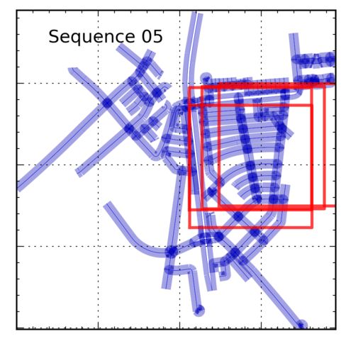
60 4.5
50 4.0
Angular Error (deg)
3.5
Position Error (m)
40 3.0
30 2.5
20 2.0
1.5
10 1.0
0 0.5 -1
10-1 100 101 102 103 10 100 101 102 103
Signal to Noise Ratio Signal to Noise Ratio
Figure 6. Localization Accuracy with Noise: Position and head-
ing error with different noise levels. Averaged over five indepen-
dent samples of noise.
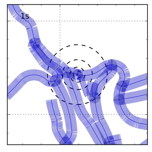
Figure 7. Ambiguous Sequences: Both 04 and 06 cannot be
Ambiguous Sequences: Sequences 04 and 06, shown in localized due to fundamental ambiguities. Sequence 04 consists
Fig. 7, are fundamentally ambiguous and cannot be local- of a short, straight driving sequence and 06 traverses a symmetric
ized with monocular, stereo or even GPS-based odometry. part of the map, resulting in two equally likely modes.
Sequence 04 is a short sequence on a straight road segment
and, in the absence of any turns, cannot be localized be- Gaussian noise to the GPS-based odometry. For each se-
yond somewhere on the long road segment. Sequence 06 is quence five different samples of noisy odometry were cre-
longer and has turns, but traverses a symmetric path which ated with signal-to-noise ratios (SNR) ranging from 0.1 to
results in a fundamental bimodality. In both cases our ap- 1000. Fig. 6 depicts error in position and heading after lo-
proach correctly indicates the set of probable locations. calization. As expected, error increases as the SNR de-
Simplification Threshold: We study the impact of vary- creases, however the performance scales well, showing little
ing the mixture model simplification threshold. Fig. 4 de- change in error until the SNR drops below 1.
picts computation time per frame and localized position er-
Scalability: Running on 16 cores with a basic Python im-
ror averaged over sequences as a function of the threshold,
plementation, we are able to achieve real time results as
ranging from 10−5 to 0.1 nats. We excluded sequences 04
shown in Fig. 4 (right). To test the ability of our method
and 06 as they are inherently ambiguous. As expected, com-
to scale to large maps we ran the sequences using stereo
putation time decreases and error increases with more sim-
odometry and a map covering the entire urban district of
plification (i.e., larger threshold). However, there is a point
Karlsruhe, Germany. This map was approximately 18km2
of diminishing returns for computation time around 10−2
and had over 2,150km of drivable road. Despite this, the
nats, and little difference in error for smaller values. Thus
errors were the same as with the smaller maps and, while
we use a threshold of 10−2 for all other experiments.
computation was slower, it still only took around 10 sec-
Map Size: To investigate the impact of region size on lo- onds per frame on average. We expect this could be greatly
calization performance, we assign uniform probability to improved with suitable optimizations. Results on sequence
portions of the map in a square region centered at the ground 02 are shown in Fig. 1 and more are available in the supple-
truth initial position and give zero initial probability to map mental material.
locations outside the region. We varied the size of the
square from 100m up to the typical map size of 2km, con- 5. Conclusions
stituting an average of 300m to 47km of drivable road. We
In this paper we have proposed an affordable approach
evaluated the time to localization for all non-ambiguous se-
to self-localization which employs (one or two) cameras
quences (i.e., all but 04, 06) and plotted the average as a
mounted on the vehicle as well as crowd sourcing in the
function of the region size in Fig. 5. As expected, small ini-
form of free online maps. We have demonstrated the ef-
tial regions allow for faster localization. Somewhat surpris-
fectiveness of our approach in a variety of diverse scenar-
ingly, after the region becomes sufficiently large, the impact
ios including highway, suburbs as well as crowded urban
on localization becomes negligible. This is due to the inher-
scenes. Furthermore, we have validated our approach on
ent uniqueness of most sufficiently long paths, even in very
the KITTI visual odometry benchmark and shown that we
large regions with many streets as the one shown in Fig. 1.
are able to localize our vehicle with a precision of 3 m
While localization in a large and truly perfect Manhattan
after only 20 seconds of driving. This is a new and ex-
world with equiangular intersections and equilength streets
citing problem for computer vision and we believe there
would be nearly impossible based purely on odometry, such
is much more to do. In particular, OpenStreetMaps con-
a world is not often realized as even Manhattan itself has
tains many other salient pieces of information to aid in
non-perpendicular roads such as Broadway!
localization such as speed limits, street names, numbers
Noise: To study the impact of noise on the localization ac- of lanes, and more; we plan to exploit this information
curacy, we synthesized odometry measurements by adding in the future. Finally, code and videos are available at
http://www.cs.toronto.edu/˜mbrubake.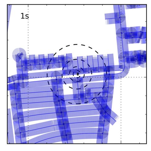
Figure 8. Selected Frames: Inference results for some of the sequences, full results can be found in the supplemental material. The left
most column shows the full map region for each sequence, followed by zoomed in sections of the map showing the posterior distribution
over time. The black line is the GPS trajectory and the concentric circles indicate the current GPS position. Grid lines are every 500m.

Acknowledgements Marcus A. Brubaker was supported by a                      27(6):647–665, 2008.
Postdoctoral Fellowship from the Natural Sciences and Engineer-         [5] F. Dellaert, W. Burgard, D. Fox, and S. Thrun. Using the con-
ing Research Council of Canada.                                             densation algorithm for robust, vision-based mobile robot lo-
                                                                            calization. CVPR, 1999.
References                                                              [6] H. Durrant-Whyte and T. Bailey. Simultaneous Localisa-
                                                                            tion and Mapping (SLAM): Part I The Essential Algorithms.
 [1] P. Alcantarilla, L. Bergasa, and F. Dellaert. Visual odometry          RAM, 2:2006, 2006.
     priors for robust EKF-SLAM. In ICRA, 2010.                         [7] D. Fox, W. Burgard, F. Dellaert, and S. Thrun. Monte carlo
 [2] G. Baatz, K. Köser, D. Chen, R. Grzeszczuk, and M. Polle-             localization: Efficient position estimation for mobile robots.
     feys. Leveraging 3D City Models for Rotation Invariant                 In AAAI, 1999.
     Place-of-Interest Recognition. IJCV, 2012.                         [8] A. Geiger, P. Lenz, and R. Urtasun. Are we ready for Au-
 [3] H. Badino, D. Huber, and T. Kanade. Real-time topometric               tonomous Driving? The KITTI Vision Benchmark Suite. In
     localization. In ICRA, May 2012.                                       CVPR, 2012.
 [4] M. Cummins and P. Newman. FAB-MAP: Probabilistic Lo-               [9] A. Geiger, J. Ziegler, and C. Stiller. Stereoscan: Dense 3d
     calization and Mapping in the Space of Appearance. IJRR,               reconstruction in real-time. In IV, 2011.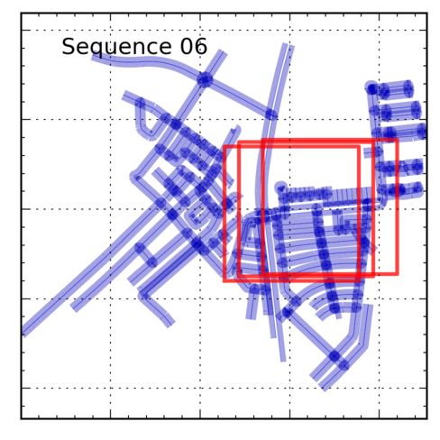
[10] J.-S. Gutmann, W. Burgard, D. Fox, and K. Konolige. An          10−8 we consider f (st−1 ) to be approximately constantly
     experimental comparison of localization methods. In ICIRS,      and the integral in Equation (10) can then be computed
     1998.                                                           analytically as f (µ)N (st |Aµ + b, Σx + AΣAT ) which
[11] J. Hays and A. A. Efros. im2gps: estimating geographic          corresponds to the prediction step of a Kalman filter. If
     information from a single image. In CVPR, 2008.                  d
                                                                     dµ g(µ, Σ) ≥ η then the mode overlaps the inflection point
[12] J. Hershey and P. Olsen. Approximating the Kullback-            of f (st−1 ) and the analytic model will not be a good ap-
     Leibler Divergence Between Gaussian Mixture Models. In
                                                                     proximation. Instead, we use a Monte Carlo approximation,
     ICASSP, volume 4, pages 317–320, 2007.                                                                 (j)
[13] M. Kaess, H. Johannsson, R. Roberts, V. Ila, J. J. Leonard,
                                                                     drawing a set of M = 400 samples st−1 ∼ N (µ, Σ) for j =
     and F. Dellaert. iSAM2: Incremental smoothing and map-          1, . . . , M and approximate the integral with a single compo-
                                                                                                          PM          (j)
     ping using the Bayes tree. IJRR, 31:217–236, 2012.              nent cN (st |µ̂, Σ̂) where c = M −1 j=1 f (st−1 ), and µ̂, Σ̂
[14] M. Kaess, K. Ni, and F. Dellaert. Flow separation for fast      are found by moment matching to the Monte Carlo mix-
                                                                                            PM        (j)            (j)
     and robust stereo odometry. In ICRA, 2009.                      ture approximation j=1 f (st−1 )N (st |Ast−1 + b, Σx ).
[15] J. Levinson, M. Montemerlo, and S. Thrun. Map-based pre-        Once the integral in Equation (10) is approximated we must
     cision vehicle localization in urban environments. In RSS,      incorporate the observation yt . Because the observations
     2007.                                                           are Gauss-Linear and the integral approximations are Gaus-
[16] Y. Li, N. Snavely, D. Huttenlocher, and P. Fua. Worldwide       sians this consists of multiplying two Gaussian distributions
     pose estimation using 3d point clouds. In ECCV, 2012.           as in the update step of the Kalman filter.
[17] C. Mei, G. Sibley, M. Cummins, P. Newman, and I. Reid.              Performing the above for each component and each pair
     Real: A system for large-scale mapping in constant-time us-     of nodes produces a set of mixture model components for
     ing stereo. IJCV, pages 1–17, 2010.
                                                                     each u, the weights of which are proportional to Put . After
[18] M. Montemerlo, S. Thrun, D. Koller, and B. Wegbreit. Fast-
                                                                     normalizing the mixtures for each street, normalizing across
     SLAM 2.0: An improved particle filtering algorithm for
     simultaneous localization and mapping that provably con-
                                                                     streets allows for the computation of Put , the probability of
     verges. In IJCAI, 2003.                                         being on a given street. The procedure for recursively up-
[19] D. Nister, O. Naroditsky, and J. R. Bergen. Visual odometry.    dating the posterior is summarized in Algorithm 1 and more
     In CVPR, 2004.                                                  details can be found in the Supplemental Material.
[20] S. M. Oh, S. Tariq, B. N. Walker, and F. Dellaert. Map-based
     priors for localization. In ICIRS, 2004.                        B. Mixture Model Simplification
[21] R. Paul and P. Newman. FAB-MAP 3D: Topological map-                                                                     f (x)       =
     ping with spatial and visual appearance. In ICRA, 2010.         P Given a Gaussian mixture model              P
                                                                        a π a N (x|µ a , Σ a ) we seek   g(x)   =     b ω b N (x|µ b , Σ b )
[22] A. Pronobis, B. Caputo, P. Jensfelt, and H. Christensen. A
                                                                     with the least number of components such that D(f kg) <
     discriminative approach to robust visual place recognition.
     In IROS, 2006.
                                                                     where D(f kg) is the KL divergence. We begin with
                                                                     g(x) = f (x) and successively remove the lowest weight
[23] A. Rottmann, O. Martı́nez Mozos, C. Stachniss, and W. Bur-
     gard. Place classification of indoor environments with mo-      component of g(x) and update the remaining components
     bile robots using boosting. In AAAI, 2005.                      to better fit f (x) so long as g(x) remains a good approx-
[24] T. Sattler, B. Leibe, and L. Kobbelt. Fast image-based local-   imation. To compute the KL divergence D(f kg), we use
     ization using direct 2d-to-3d matching. In ICCV, 2011.          instead a variational upper bound [12]. Introducing the
[25] S. Se, D. Lowe, and J. Little. Mobile robot localization and    variational parameters φa,b ≥ 0 and ψa,b ≥ 0 such that
                                                                     P                      P
     mapping with uncertainty using scale-invariant visual land-        b φa,b = πa and        a ψa,b
                                                                                                   P
                                                                                                      = ωb , D(f kg) ≤ D̂(φ, ψ, f, g)
     marks. IJRR, 21:735–758, 2002.                                                                                 φa,b
                                                                     where D̂(φ, ψ, f, g) =           a,b φa,b (log ψa,b + D(fa kgb ))
[26] B. Williams, M. Cummins, J. Neira, P. Newman, I. Reid,          and D(fa kgb ) is the KL divergence between N (x|µa , Σa )
     and J. Tardós. A comparison of loop closing techniques in
                                                                     and N (x|µb , Σb ). To compute the upper bound of D(f kg)
     monocular SLAM. RAS, 2009.
                                                                     we minimize D̂(φ, ψ, f, g) with respect to the variational
[27] J. Wu and J. M. Rehg. Where am I: Place instance and cate-
     gory recognition using spatial PACT. In CVPR, 2008.
                                                                     parameters φ and ψ. Similarly, to update the components of
                                                                     g we minimize D̂(φ, ψ, f, g) with respect to the variational
                                                                     parameters φ and ψ as well as the parameters ωb , µb and
A. Inference Details
                                                                     Σb . While this objective function is non-convex, for each
    To measure whether f (st−1 ) = p(ut |xt−1 ) is constant          set of parameters individually the exact minima can be
for a mixture component
                      R     N (µ(i) , Σ(i) ) we consider the         found, providing an efficient coordinate-descent algorithm.
function g(µ, Σ) = f (st−1 )N (st−1 |µ, Σ)dst−1 which,               The update equations for φ, ψ, ωb , µb and Σb , along
in the case of the Gaussian CDF form of f (st−1 ) can be             with the details of their derivation and a summary of the
shown to be a Gaussian CDF (proof in Supplementary Ma-               algorithm are found in the Supplementary Material.
                                      d
terial). Dropping the index, i, if k dµ g(µ, Σ)k < η for η =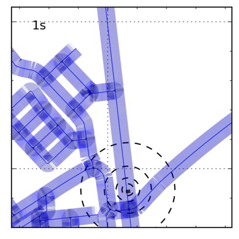
You can also read