Do We Need to Compensate for Motion Distortion and Doppler Effects in Spinning Radar Navigation?
←
→
Page content transcription
If your browser does not render page correctly, please read the page content below
IEEE ROBOTICS AND AUTOMATION LETTERS, VOL. 6, NO. 2, APRIL 2021                                                                                             771

   Do We Need to Compensate for Motion Distortion
   and Doppler Effects in Spinning Radar Navigation?
                                 Keenan Burnett , Angela P. Schoellig , and Timothy D. Barfoot

   Abstract—In order to tackle the challenge of unfavorable
weather conditions such as rain and snow, radar is being revisited
as a parallel sensing modality to vision and lidar. Recent works
have made tremendous progress in applying spinning radar to
odometry and place recognition. However, these works have so far
ignored the impact of motion distortion and Doppler effects on
spinning-radar-based navigation, which may be significant in the
self-driving car domain where speeds can be high. In this work,
we demonstrate the effect of these distortions on radar odometry
using the Oxford Radar RobotCar Dataset and metric localiza-
tion using our own data-taking platform. We revisit a lightweight
estimator that can recover the motion between a pair of radar
scans while accounting for both effects. Our conclusion is that
both motion distortion and the Doppler effect are significant in
different aspects of spinning radar navigation, with the former
more prominent than the latter. Code for this project can be found
at: https://github.com/keenan-burnett/yeti_radar_odometry
                                                                                  Fig. 1. Our data-taking platform, Boreas, which includes a Velodyne Alpha-
   Index Terms—Localization,              range      sensing,     intelligent
                                                                                  Prime (128-beam) lidar, Navtech CIR204-H radar, FLIR Blackfly S monocular
transportation systems.                                                           camera, and Applanix POSLV GNSS.

                            I. INTRODUCTION                                          Recent works have made tremendous progress in
                                                                                  applying the Navtech radar to odometry [2]–[7] and place
       S RESEARCHERS continue to advance the capabilities of
A      autonomous vehicles, attention has begun to shift towards
inclement weather conditions. Currently, most autonomous ve-
                                                                                  recognition [8]–[10]. However, all of these works make the
                                                                                  simplifying assumption that a radar scan is collected at a
                                                                                  single instant in time. In reality, the sensor is rotating while the
hicles rely primarily cameras and lidar for perception and lo-                    vehicle is moving causing the radar scan to be distorted in a
calization. Although these sensors have been shown to achieve                     cork-screw fashion. Range measurements of the Navtech radar
sufficient performance under nominal conditions, rain and snow                    are also impacted by Doppler frequency shifts resulting from
remain an open problem. Radar sensors, such as the one pro-                       the relative velocity between the sensor and its surroundings.
duced by Navtech [1], may provide a solution.                                     Both distortion effects become more pronounced as the speed
   Due to its longer wavelength, radar is robust to small particles               of the ego-vehicle increases. Most automotive radar sensors are
such as dust, fog, rain, or snow, which can negatively impact                     not impacted by either distortion effect. However, the Navtech
cameras and lidar sensors. Furthermore, radar sensors tend to                     provides 360◦ coverage with accurate range and azimuth
have a longer detection range and can penetrate through some                      resolution, making it an appealing navigation sensor.
materials allowing them to see beyond the line of sight of lidar.                    In this paper, we demonstrate the effect that motion distortion
These features make radar particularly well-suited for inclement                  can have on radar-based navigation. We also revisit a lightweight
weather. However, radar sensors have coarser spatial resolution                   estimator, Motion-Compensated RANSAC [11], which can re-
than lidar and suffer from a higher noise floor making them                       cover the motion between a pair of scans and remove the
challenging to work with.                                                         distortion. The Doppler effect was briefly acknowledged in [2]
                                                                                  but our work is the first to demonstrate the impact on radar-based
   Manuscript received October 15, 2020; accepted January 13, 2021. Date of       navigation and to provide a method for its compensation.
publication January 18, 2021; date of current version February 1, 2021. This         As our primary experiment to demonstrate the effects of
letter was recommended for publication by Associate Editor J. L. Blanco-Claraco   motion distortion, we perform radar odometry on the Oxford
and Editor J. Civera upon evaluation of the reviewers’ comments. (Correspond-
ing author: Keenan Burnett.)                                                      Radar RobotCar Dataset [12]. As an additional experiment, we
   The authors are with the University of Toronto Institute for                   perform metric localization using our own data-taking platform,
Aerospace Studies (UTIAS), Toronto, Ontario M4Y2X6, Canada (e-mail:               shown in Fig. 1. Qualitative results of both distortion effects
keenan.burnett@robotics.utias.utoronto.ca;         schoellig@utias.utoronto.ca;
tim.barfoot@utoronto.ca).                                                         are also provided. Rather than focusing on achieving state-of-
   Digital Object Identifier 10.1109/LRA.2021.3052439                             the-art navigation results, the goal of this paper is to show that
                         2377-3766 © 2021 IEEE. Personal use is permitted, but republication/redistribution requires IEEE permission.
                                       See https://www.ieee.org/publications/rights/index.html for more information.

         Authorized licensed use limited to: The University of Toronto. Downloaded on April 27,2021 at 20:40:05 UTC from IEEE Xplore. Restrictions apply.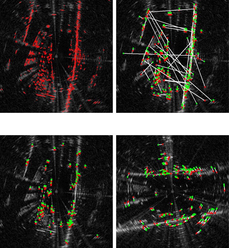
772                                                                                     IEEE ROBOTICS AND AUTOMATION LETTERS, VOL. 6, NO. 2, APRIL 2021

motion distortion and Doppler effects are significant and can be                 are ignored by the scan matching. This approach currently
compensated for with relative ease.                                              represents the state of the art for radar odometry performance.
   The rest of this paper is organized as follows: Section II                       Still others focus on topological localization that can be used
discusses related work, III provides our methodology to match                    by downstream metric mapping and localization systems to
two radar scans while compensating for motion distortion and                     identify loop closures. Săftescu et al. [8] learn a metric space
the Doppler effect, IV has experiments, and V concludes.                         embedding for radar scans using a convolutional neural network.
                                                                                 Nearest-neighbour matching is then used to recognize locations
                                                                                 at test time. Gadd et al. [9] improve this place recognition
                         II. RELATED WORK                                        performance by integrating a rotationally invariant metric space
   Self-driving vehicles designed to operate in ideal conditions                 embedding into a sequence-based trajectory matching system
often relegate radar to a role as a secondary sensor as part of an               previously applied to vision. In [23], Tang et al. focus on
emergency braking system [13]. However, recent advances in                       localization between a radar on the ground and overhead satellite
Frequency Modulated Continuous Wave (FMCW) radar indicate                        imagery.
that it is a promising sensor for navigation and other tasks                        Other recent works using a spinning radar include the work
typically reserved for vision and lidar. Jose and Adams [14]                     by Weston et al. [24] that learns to generate occupancy grids
[15] were the first to research the application of spinning radar                from raw radar scans by using lidar data as ground truth. Kaul
to outdoor SLAM. In [16], Checchin et al. present one of the                     et al. [25] train a semantic segmentation model for radar data
first mapping and localization systems designed for a FMCW                       using labels derived from lidar- and vision-based semantic seg-
scanning radar. Their approach finds the transformation between                  mentation.
pairs of scans using the Fourier Mellin transform. Vivet et al. [17]                Motion distortion has been treated in the literature through the
were the first to address the motion distortion problem for                      use of continuous-time trajectory estimation [11], [26]–[29] for
scanning radar. Our approach to motion distortion is simpler and                 lidars [30] and rolling-shutter cameras [31], but these tools are
we offer a more up-to-date analysis on a dataset that is relevant                yet to be applied to spinning radar. TEASER [32] demonstrates
to current research. In [18], Kellner et al. present a method                    a robust registration algorithm with optimality guarantees. How-
that estimates the linear and angular velocity of the ego-vehicle                ever, it assumes that pointclouds are collected at single instances
when the Doppler velocity of each target is known. The use of                    in time. Thus, TEASER is impacted by motion distortion in the
single-chip FMCW radar has recently become a salient area of                     same manner as rigid RANSAC.
research for robust indoor positioning systems under conditions                     Our work focuses on the problem of motion distortion and
unfavorable to vision [19], [20].                                                Doppler effects using the Navtech radar sensor which has not
   In [2], Cen et al. present their seminal work that has rekindled              received attention from these prior works. Ideally, our findings
interest in applying FCMW radar to navigation. Their work                        will inform future research in this area looking to advance the
presented a new method to extract stable keypoints and perform                   state of the art in radar-based navigation.
scan matching using graph matching. Further research in this
area has been spurred by the introduction of the Oxford Radar                                               III. METHODOLOGY
RobotCar Dataset [12], which includes lidar, vision, and radar
                                                                                   Section III-A describes our approach to feature extraction
data from a Navtech radar. Other radar-focused datasets include
                                                                                 and data association. In Section III-B, we describe a motion-
the MulRan place recognition dataset [10] and the RADIATE
                                                                                 compensated estimator and a rigid estimator for comparison.
object detection dataset [21].
                                                                                 Section III-C explains how the Doppler effect impacts radar
   Odometry has recently been a central focus of radar-based
                                                                                 range measurements and how to compensate for it.
navigation research. Components of an odometry pipeline can
be repurposed for mapping and localization, which is an ultimate
                                                                                 A. Feature Extraction
goal of this research. In [3], Cen et al. present an update to
their radar odometry pipeline with improved keypoint detec-                         Feature detection in radar data is more challenging than in
tion, descriptors, and a new graph matching strategy. Aldera                     lidar or vision due to its higher noise floor and lower spatial
et al. [4] train a focus of attention policy to downsample the                   resolution. Constant False Alarm Rate (CFAR) [33] is a simple
measurements given to data association, thus speeding up the                     feature detector that is popular for use with radar. CFAR is
odometry pipeline. In [6], Barnes and Posner present a deep-                     designed to estimate the local noise floor and capture relative
learning-based keypoint detector and descriptor that are learned                 peaks in the radar data. One-dimensional CFAR can be applied to
directly from radar data using differentiable point matching                     Navtech data by convolving each azimuth with a sliding-window
and pose estimation. In [22], Hong et al. demonstrate the first                  detector.
radar-SLAM pipeline capable of handling extreme weather.                            As discussed in [2], CFAR is not the best detector for radar-
   Other approaches forego the feature extraction process and                    based navigation. CFAR produces many redundant keypoints,
instead use the entire radar scan for correlative scan matching.                 is difficult to tune, and produces false positives due to the noise
Park et al. [7] use the Fourier Mellin Transform on Cartesian                    artifacts present in radar. Instead, Cen et al. [2] proposed a
and log-polar radar images to sequentially estimate rotation and                 detector that estimates a signal’s noise statistics and then scales
translation. In [5], Barnes et al. present a fully differentiable,               the power at each range by the probability that it is a real
correlation-based radar odometry approach. In their system, a                    detection. In [3], Cen et al. proposed an alternative detector
binary mask is learned such that unwanted distractor features                    that identifies continuous regions of the scan with high intensity

       Authorized licensed use limited to: The University of Toronto. Downloaded on April 27,2021 at 20:40:05 UTC from IEEE Xplore. Restrictions apply.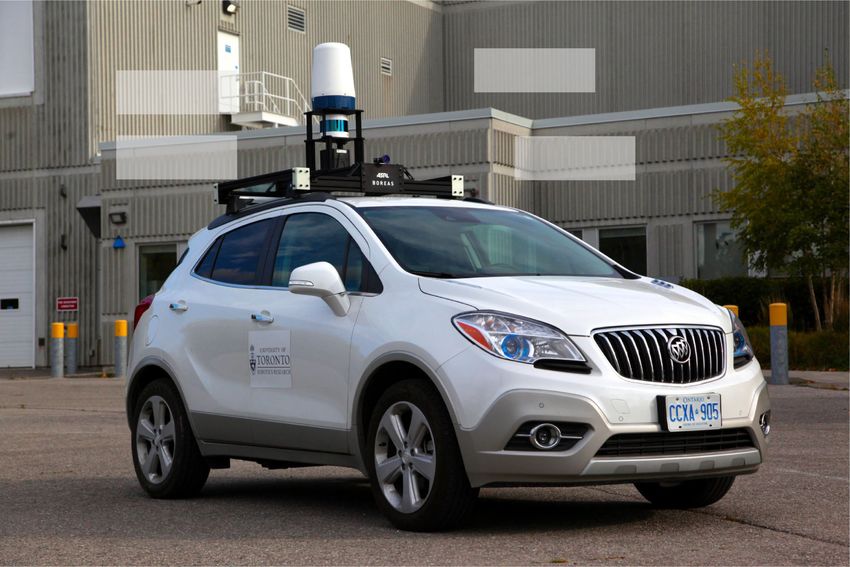
BURNETT et al.: DO WE NEED TO COMPENSATE FOR MOTION DISTORTION AND DOPPLER EFFECTS IN SPINNING RADAR NAVIGATION?                                            773

                                                                                    shows the result of the initial data association. Note that there
                                                                                    are several outliers. Fig. 2(c), (d) shows the remaining inliers
                                                                                    after performing RANSAC.

                                                                                    B. Motion Distortion
                                                                                       The output of data association is not perfect and often contains
                                                                                    outliers. As a result, it is common to employ an additional
                                                                                    outlier rejection scheme during estimation. In this paper, we use
                                                                                    RANSAC [36] to find an outlier-free set that can then be used to
                                                                                    estimate the desired transform. If we assume that two radar scans
                                                                                    are taken at times t̄1 and t̄2 , then the transformation between
                                                                                    them can be estimated directly using the approach described
                                                                                    in [37].
                                                                                       During each iteration of RANSAC, a random subset of size
                                                                                    S is drawn from the initial matches and a candidate transform is
                                                                                    generated. If the number of inliers exceeds a desired threshold
                                                                                    or a maximum number of iterations is reached, the algorithm
                                                                                    terminates. Radar scans are 2D and as such we use S = 2. The
                                                                                    estimation process is repeated on the largest inlier set to obtain a
                                                                                    more accurate transform. We will refer to this approach as rigid
                                                                                    RANSAC.
                                                                                       Our derivation of motion-compensated RANSAC follows
                                                                                    closely from [11]. However, we are applying the algorithm to a
Fig. 2. This figure illustrates our feature extraction and matching process.        scanning radar in 2D instead of a two-axis scanning lidar in 3D.
(a) displays our raw extracted features. (b) displays the output of our ORB-        Furthermore, our derivation is shorter and uses updated notation
descriptor-based data association. (c) and (d) show the inlier set resulting from   from [38].
motion-compensated RANSAC while driving straight and rotating.
                                                                                       The principal idea behind motion-compensated RANSAC is
                                                                                    to estimate the velocity of the sensor instead of estimating a
                                                                                    transformation. We make the simplifying assumption that the
and low gradients. Keypoints are then extracted by locating
                                                                                    linear and angular velocity between a pair of scans is constant.
the middle of each continuous region. We will refer to these
                                                                                    The combined velocity vector  is defined as
detectors as Cen2018 and Cen2019, respectively.
   The original formulations of these detectors did not lend                                                            ν
themselves to real-time operation. As such, we made several                                                    =           ,                        (1)
                                                                                                                        ω
modifications to improve the runtime. For Cen2018, we use a
Gaussian filter instead of a binomial filter, and we calculate the                  where ν and ω are the linear and angular velocity in the sensor
mean of each azimuth instead of using a median filter. We do                        frame. To account for motion distortion, we remove the assump-
not remove multipath reflections.                                                   tion that radar scans are taken at a single instant in time. Data
   Cen2019 was designed to be easier to tune and have less                          association produces two sets of corresponding measurements,
redundant keypoints. However, we found that by adjusting the                        ym,1 and ym,2 , where m = 1. . .M . Each pair of features, m, is
probability threshold of detections, Cen2018 obtained better                        extracted from sequential radar frames 1 and 2 at times tm,1 and
odometry performance when combined with our RANSAC-                                 tm,2 . The temporal difference between a pair of measurements is
based scan matching. Based on these preliminary tests, we                           Δtm := tm,2 − tm,1 . The generative model for measurements
concluded that Cen2018 was the best choice for our experiments.                     is given as
Fig. 2(a) shows Cen2018 features plotted on top of a Cartesian                                      ym,1 := f (Ts (tm,1 )pm ) + nm,1 ,
radar image.
   We convert the raw radar scans output by the Navtech sensor,                                     ym,2 := f (Ts (tm,2 )pm ) + nm,2 ,                      (2)
which are in polar form, into Cartesian form. We then calculate                     where f (·) is a nonlinear transformation from Cartesian to
an ORB descriptor [34] for each keypoint on the Cartesian                           cylindrical coordinates and Ts (t) is a 4 x 4 homogeneous
image. There may be better keypoint descriptors for radar data,                     transformation matrix representing the pose of the sensor frame
such as the learned feature descriptors employed in [6]. However,                   Fs with respect to the inertial frame Fi at time t. pm is the

ORB descriptors are quick to implement, rotationally invariant,                     original landmark location in the inertial frame. We assume
and resistant to noise.                                                             that each measurement is corrupted by zero-mean Gaussian
   For data association, we perform brute-force matching of                         noise: nm,1 ∼ N (0, Rm,1 ). The transformation between a pair
ORB descriptors. We then apply a nearest-neighbor distance                          of measurements is defined as
ratio test [35] in order to remove false matches. The remaining
matches are sent to our RANSAC-based estimators. Fig. 2(b)                                             Tm := Ts (tm,2 )Ts (tm,1 )−1 .                       (3)

         Authorized licensed use limited to: The University of Toronto. Downloaded on April 27,2021 at 20:40:05 UTC from IEEE Xplore. Restrictions apply.
774 IEEE ROBOTICS AND AUTOMATION LETTERS, VOL. 6, NO. 2, APRIL 2021
To obtain our objective function, we convert feature locations
from polar coordinates into local Cartesian coordinates:
pm,2 = f −1 (ym,2 ), (4)
pm,1 = f −1 (ym,1 ). (5)
We then use the local transformation Tm to create a pseudomea-
surement p̂m,2 ,
Fig. 3. This diagram illustrates the relationship between the ego-motion (v, ω)
and the radial velocity u.
p̂m,2 = Tm pm,1 . (6)
operating point. We can rewrite gm () as:
The error is then defined in the sensor coordinates and summed
over each pair of measurements to obtain our objective function: gm () = exp(Δtm δ ∧ )Tm pm,1 ,
em = pm,2 − p̂m,2 , (7) ≈ (1 + Δtm δ ∧ )Tm pm,1 , (14)
where we use an approximation for small pose changes. We
1 T −1
M
swap the order of operations using the (·) operator [38]:
J() := e R em . (8)
2 m=1 m cart,m gm () = Tm pm,1 + Δtm (Tm pm,1 ) δ
Here we introduce some notation for dealing with transforma- = gm + Gm δ, (15)
tion matrices in SE(3). A transformation T ∈ SE(3) is related
to its associated Lie algebra ξ ∧ ∈ se(3) through the exponential ρ η1 −ρ∧
p = = T . (16)
map: η 0 0T
We can now rewrite the error function from (7):
C r
T= T = exp(ξ ∧ ), (9) em ≈ pm,2 − gm − Gm δ
0 1
= em − Gm δ. (17)
where C is 3 × 3 a rotation matrix, r is a 3 × 1 translation By inserting this equation for the error function into the ob-
vector, and (·)∧ is an overloaded operator that converts a vector jective function from (8), and taking the derivative with respect
of rotation angles φ into a member of so(3) and ξ into a member to the perturbation and setting it to zero, ∂J() = 0, we obtain
∂δ T
of se(3): the optimal update:
⎡⎤∧ ⎡ ⎤
−1
φ1 0 −φ3 φ2
⎢ ⎥ ⎢ ⎥ δ =
GTm R−1
cart,m Gm GTm R−1
cart,m em ,
φ∧ = ⎣φ2 ⎦ := ⎣ φ3 0 −φ1 ⎦ , (10) m m
φ3 −φ2 φ1 0 (18)
∧ where Rcart,m = Hm Rm,2 HTm is the covariance in the local
ρ φ∧ ρ Cartesian frame, h(·) = f −1 (·), and Hm = ∂h ∂x |gm . The opti-
∧
ξ = := T . (11)
φ 0 1 mal perturbation δ is used in a Gauss-Newton optimization
scheme and the process repeats until converges.
Given our constant-velocity assumption, we can convert from This method allows us to estimate the linear and angular
a velocity vector into a transformation matrix using the velocity between a pair of radar scans directly while accounting
following formula: for motion distortion. These velocity estimates can then be used
to remove the motion distortion from a measurement relative
T = exp(Δt ∧ ). (12) to a reference time using (12). MC-RANSAC is intended to
be a lightweight method for showcasing the effects of motion
In order to optimize our objective function J(), we first distortion. A significant improvement to this pipeline would be to
need to derive the relationship between Tm and . The velocity use the inliers of MC-RANSAC as an input to another estimator,
vector can be written as the sum of a nominal velocity and such as [28]. The inliers could also be used for mapping and
a small perturbation δ. This lets us rewrite the transformation localization or SLAM.
Tm as the product of a nominal transformation Tm and a small
perturbation δTm :
C. Doppler Correction
∧
Tm = exp(Δtm ( + δ) ) = δTm Tm . (13) In order to compensate for Doppler effects, we need to know
the linear velocity of the sensor v. This can either be obtained
Let gm () := Tm pm,1 , which is nonlinear due to the trans- from a GPS/IMU or using one of the estimators described above.
formation. Our goal is to linearize gm () about a nominal As shown in Fig. 3, the motion of the sensor results in an apparent
Authorized licensed use limited to: The University of Toronto. Downloaded on April 27,2021 at 20:40:05 UTC from IEEE Xplore. Restrictions apply.BURNETT et al.: DO WE NEED TO COMPENSATE FOR MOTION DISTORTION AND DOPPLER EFFECTS IN SPINNING RADAR NAVIGATION? 775
factor:
Δrcorr = β(vx cos(φ) + vy sin(φ)). (21)
We use this simple correction in all our experiments with the
velocity (vx , vy ) coming from our motion estimator.
IV. EXPERIMENTAL RESULTS
In order to answer the question posed by this paper, we have
devised two experiments. The first is to compare the perfor-
mance of rigid RANSAC and MC-RANSAC (with or without
Doppler corrections) on radar odometry using the Oxford Radar
RobotCar Dataset [12]. The second experiment demonstrates
Fig. 4. This figure depicts the sawtooth modulation pattern of an FMCW radar.
The transmitted signal is blue and the received signal is red. the impact of both distortion effects on localization using our
own data. We also provide qualitative results demonstrating both
relative velocity between the sensor and its surrounding envi- distortion effects.
ronment. This relative velocity causes the received frequency The Navtech radar is a frequency modulated continuous wave
to be altered according to the Doppler effect. Note that only the (FMCW) radar. For each azimuth, the sensor outputs the re-
radial component of the velocity u = vx cos(φ) + vy sin(φ) will ceived signal power at each range bin. The sensor spins at 4 Hz
result in a Doppler shift. The Radar Handbook by Skolnik [39] and provides 400 measurements per rotation with a 163 m range,
provides an expression for the Doppler frequency: 4.32 cm range resolution, 1.8◦ horizontal beamwidth, and 0.9◦
azimuth resolution.
2u
fd = , (19) The Oxford Radar RobotCar Dataset is an autonomous driv-
λ ing dataset that includes two 32-beam lidars, six cameras, a
where λ is the wavelength of the signal. Note that for an object GPS/IMU, and the Navtech sensor. The dataset includes thirty-
moving towards the radar (u > 0) or vice versa, the Doppler fre- two traversals equating to 280 km of driving in total.
quency will be positive resulting in a higher received frequency.
For FMCW radar such as the Navtech sensor, the distance to A. Odometry
a target is determined by measuring the change in frequency
between the received signal and the carrier wave Δf : Our goal is to make a fair comparison between two estimators
where the main difference is the compensation of distortion
cΔf
r= , (20) effects. To do this, we use the same number of maximum
2(df /dt) iterations (100), and the same inlier threshold (0.35 m) for both
where df /dt is the slope of the modulation pattern used by the rigid RANSAC and MC-RANSAC. We also fix the random seed
carrier wave and c is the speed of light. FMCW radar require before running either estimator to ensure that the differences in
two measurements to disentangle the frequency shift resulting performance are not due to the random selection of subsets.
from range and relative velocity. Since the Navtech sensor scans For feature extraction, we use the same setup parameters
each azimuth only once, the measured frequency shift is the for Cen2018 as in [2] except that we use a higher probability
combination of both the range difference and Doppler frequency. threshold, zq = 3.0, and a Gaussian filter with σ = 17 range
From Fig. 4, we can see that a positive Doppler frequency fd bins. We convert polar radar scans into a Cartesian image with
will result in an increase in the received frequency and in turn 0.2592 m per pixel and a width of 964 pixels (250 m). For
a reduction in the observed frequency difference Δf . Thus, a ORB descriptors, we use a patch size of 21 pixels (5.4 m).
positive Doppler frequency will decrease the apparent range of For data association, we use a nearest-neighbor distance ratio
a target. of 0.8. For Doppler corrections, we use β = 0.049. For each
The Navtech radar operates between 76 GHz and 77 GHz radar scan, extracting Cen2018 features takes approximately
resulting in a bandwidth of 1 GHz. Navtech states that they 35 ms. Rigid RANSAC runs in 1-2 ms and MC-RANSAC in
use a sawtooth modulation pattern. Given 1600 measurements 20-50 ms. Calculating orb descriptors takes 5 ms and brute-force
per second and assuming the entire bandwidth is used for each matching takes 15 ms. These processing times were obtained on
measurement, df /dt ≈ 1.6 × 10¹² . a quad-core Intel Xeon E3-1505 M 3.0 GHz CPU with 32 GB
Hence, if the forward velocity of the sensor is 1 m/s, a of RAM.
target positioned along the x-axis (forward) of the sensor would Odometry results are obtained by compounding the frame-to-
experience a Doppler frequency shift of 510 Hz using (19). This frame scan matching results. Note that we do not use a motion
increase in the frequency of the received signal would decrease prior or perform additional smoothing on the odometry. Three
the apparent range to the target by 4.8 cm using (20). Naturally, sequences were used for parameter tuning. The remaining 29
this effect becomes more pronounced as the velocity increases. sequences are used to provide test results.
Let β = ft /(df /dt) where ft is the transmission frequency Table I summarizes the results of the odometry experiment.
(ft ≈ 76.5 GHz). In order to correct for the Doppler distortion, We use KITTI-style odometry metrics [40] to quantify the
the range of each target needs to be corrected by the following translational and rotational drift as is done in [6]. The metrics
Authorized licensed use limited to: The University of Toronto. Downloaded on April 27,2021 at 20:40:05 UTC from IEEE Xplore. Restrictions apply.776 IEEE ROBOTICS AND AUTOMATION LETTERS, VOL. 6, NO. 2, APRIL 2021
TABLE I
RADAR ODOMETRY RESULTS. *ODOMETRY RESULTS FROM [6]
Fig. 6. This figure highlights the impact that motion distortion can have on
the accuracy of radar-based odometry. Note that motion-compensated RANSAC
(MC-RANSAC) is much closer to the ground truth.
B. Localization
The purpose of this experiment is to demonstrate the impact of
motion distortion and Doppler effects on metric localization. As
opposed to the previous experiment, we localize between scans
taken while driving in opposite directions. While the majority of
the Oxford Radar dataset was captured at low speeds (0–10 m/s),
in this experiment we only use radar frames where the ego-
vehicle’s speed was above 10 m/s. For this experiment, we use
our own data-taking platform, shown in Fig. 1, which includes a
Velodyne Alpha-Prime lidar, Navtech CIR204-H radar, Blackfly
Fig. 5. This figure provides our KITTI-style odometry results on the Oxford S camera, and an Applanix POSLV GNSS. Individuals interested
dataset. We provide our translational and rotational drift as a function of path in using this data can fill out a Google form to gain access.1
length and speed. MC-RANSAC: motion-compensated RANSAC, MC+DOPP: Ground truth for this experiment was obtained from a 10 km
motion and distortion compensated.
drive using post-processed GNSS data provided by Applanix,
which has an accuracy of 12 cm in this case. Radar scans were
initially matched by identifying pairs of proximal scans on the
are obtained by averaging the translational and rotational drifts
outgoing and return trips based on GPS data. The Navtech
for all subsequences of lengths (100, 200, … , 800) meters.
timestamps were synchronized to GPS time to obtain an accurate
The table shows that motion-compensated RANSAC results in
position estimate.
a 9.4% reduction in translational drift and a 15.6% reduction
Our first observation was that localizing against a drive in
in rotational drift. This shows that compensating for motion
reverse is harder than odometry. When viewed from different
distortion has a modest impact on radar odometry. The table
angles, objects have different radar cross sections, which causes
also indicates that Doppler effects have a negligible impact on
them to appear differently. As a consequence, radar scans may
odometry. Our interpretation is that Doppler distortion impacts
lose or gain features when pointed in the opposite direction. This
sequential radar scans similarly such that scan registration is
change in the radar scan’s appearance was sufficient to prevent
minimally impacted.
ORB features from matching.
It should be noted that a large fraction of the Oxford dataset
As a replacement for ORB descriptors, we turned to the Radial
was collected at low speeds (0–5 m/s). This causes the motion
Statistics Descriptor (RSD) described in [2], [3]. Instead of
distortion and Doppler effects to be less noticeable.
calculating descriptors based on the Cartesian radar image, RSD
Fig. 5 depicts the translational and rotational drift of each
operates on a binary Cartesian grid derived from the detected
method as a function of path length and speed. It is clear that mo-
feature locations. This grid can be thought of as a radar target
tion compensation improves the odometry performance across
occupancy grid. For each keypoint, RSD divides the binary grid
most cases. Interestingly, MC-RANSAC does not increase in
into M azimuth slices and N range bins centered around the
error as much as rigid RANSAC as the path length increases.
keypoint. The number of keypoints (pixels) in each azimuth slice
Naturally, we would expect rigid RANSAC to become much
and range bin is counted to create two histograms. In [3], a fast
worse than MC-RANSAC at higher speeds. However, what we
Fourier transform of the azimuth histogram is concatenated with
observe is that as the speed of the vehicle increases, the motion
a normalized range histogram to form the final descriptor.
tends to become more linear. When the motion of the vehicle
In our experiment, we found that the range histogram was
is mostly linear, the motion distortion does not impact rigid
sufficient on its own, with the azimuth histogram offering only
RANSAC as much. Fig. 6 compares the odometry output of both
estimators against ground truth. The results further illustrate that
compensating for motion distortion improves performance. 1 [Online]. Available: https://forms.gle/ZGtQhKRXkxmcAGih9
Authorized licensed use limited to: The University of Toronto. Downloaded on April 27,2021 at 20:40:05 UTC from IEEE Xplore. Restrictions apply.BURNETT et al.: DO WE NEED TO COMPENSATE FOR MOTION DISTORTION AND DOPPLER EFFECTS IN SPINNING RADAR NAVIGATION? 777
TABLE II
METRIC LOCALIZATION RESULTS
Fig. 7. By compensating for motion distortion alone (MC) or both motion and
Doppler distortion (MC + DOPP), metric localization improves.
a minor improvement. It should be noted that these descriptors
are more expensive to compute (60 ms) and match (30 ms) than
ORB descriptors. These processing times were obtained using
the same hardware as in Section IV-A.
The results of our localization experiment are summarized in
Table II. In each case, we are using our RANSAC estimator from
Section III. The results in the table are obtained by calculating
the median translation and rotation error. Compensating for mo-
tion distortion results in a 41.7% reduction in translation error.
Compensating for Doppler effects results in a further 67.7%
reduction in translation error. Together, compensating for both
effects results in a 81.2% reduction in translation error. Note that
the scan-to-scan translation error is larger than in the odometry
Fig. 8. Lidar points are shown in red, radar targets are shown in green, vehicles
experiment due to the increased difficulty of localizing against are boxed in blue. (a) Both motion distortion and Doppler effects and present
a reverse drive. Fig. 7 depicts a histogram of the localization in the radar scan. (b) Motion distortion and Doppler effects have been removed
errors in this experiment. from the radar data. Note that static objects (highlighted by yellow arrows) align
much better in (b). Some of the moving vehicles (boxed in blue) are less aligned
after removing distortion. Here we do not know the other vehicles’ velocities
C. Qualitative Results and therefore the true relative velocity with respect to the ego-vehicle.
In this section, we present qualitative results of removing
note that some of the moving vehicles (boxed in blue) are less
motion distortion and Doppler effects from radar data. In Fig. 8,
aligned after removing distortion. Here we do not know the other
we have plotted points from our Velodyne lidar in red and
vehicles’ velocities and therefore the true relative velocity with
extracted radar targets in green. In this example, the ego-vehicle
respect to the ego-vehicle. These results indicate that additional
is driving at 15 m/s with vehicles approaching from the opposite
velocity information for each object is required in order to align
direction on the left-hand side of the road. In order to directly
dynamic objects. We leave this problem for future work.
compare lidar and radar measurements, we have aligned each
sensor’s output spatially and temporally using post-processed
GPS data and timestamps. Motion distortion is removed from V. CONCLUSION
the lidar points before the comparison is made. We use the lidar For the problem of odometry, compensating for motion dis-
measurements to visualize the amount of distortion present in tortion had a modest impact of reducing translational drift by
the radar scan. Fig. 8(a) shows what the original alignment looks 9.4%. Compensating for Doppler effects had a negligible effect
like when the radar scan is distorted. Fig. 8(b) shows what the on odometry performance. We postulate that Doppler effects are
alignment looks like after compensating for motion distortion negligible for odometry because their effects are quite similar
and Doppler effects. Note that static objects such as trees align from one frame to the next. In our localization experiment, we
much better with the lidar data in Fig. 8(b). It interesting to observed that compensating for motion distortion and Doppler
Authorized licensed use limited to: The University of Toronto. Downloaded on April 27,2021 at 20:40:05 UTC from IEEE Xplore. Restrictions apply.778 IEEE ROBOTICS AND AUTOMATION LETTERS, VOL. 6, NO. 2, APRIL 2021
effects reduced translation error by 41.7% and 67.7% respec- [14] E. Jose and M. D. Adams, “Relative radar cross section based feature
tively with a combined reduction of 81.2%. We also provided identification with millimeter wave radar for outdoor slam,” in Proc.
IEEE/RSJ Int. Conf. Intell. Robots Syst., vol. 1, 2004, pp. 425–430.
qualitative results demonstrating the impact of both distortion [15] E. Jose, M. Adams, J. S. Mullane, and N. M. Patrikalakis, “Predicting
effects. We noted that the velocity of each dynamic object is millimeter wave radar spectra for autonomous navigation,” IEEE Sensors
required in order to properly undistort points associated with J., vol. 10, no. 5, pp. 960–971, May 2010.
[16] P. Checchin, F. Gérossier, C. Blanc, R. Chapuis, and L. Trassoudaine,
dynamic objects. In summary, the Doppler effect can be safely “Radar scan matching slam using the Fourier-Mellin transform,” in Field
ignored for the radar odometry problem but motion distortion and Service Robotics, Berlin, Germany: Springer, 2010, pp. 151–161.
should be accounted for to achieve the best results. For metric [17] D. Vivet, P. Checchin, and R. Chapuis, “Localization and mapping
using only a rotating FMCW radar sensor,” Sensors, vol. 13, no. 4,
localization, especially for localizing in the opposite direction pp. 4527–4552, 2013.
from which the map was built, both motion distortion and [18] D. Kellner, M. Barjenbruch, J. Klappstein, J. Dickmann, and K. Dietmayer,
Doppler effects need to be compensated. Accounting for these “Instantaneous ego-motion estimation using doppler radar,” in Proc. 16th
Int. IEEE Conf. Intell. Transp. Syst., 2013, pp. 869–874.
effects is computationally cheap, but requires an accurate esti- [19] A. Kramer, C. Stahoviak, A. Santamaria-Navarro, A.-A. Agha-
mate of the linear and angular velocity of the sensor. mohammadi, and C. Heckman, “Radar-inertial ego-velocity estimation
For future work, we will investigate applying more powerful for visually degraded environments,” in Proc. IEEE Int. Conf. Robot.
Automat., 2020, pp. 5739–5746.
estimators such as [28] to odometry and the full mapping and [20] C. X. Lu et al., “Milliego: Single-chip mmwave radar aided egomotion es-
localization problem. We will also investigate learned features timation via deep sensor fusion,” in Proc. 18th Conf. Embedded Networked
and the impact of seasonal changes on radar maps. Sensor Syst., 2020, pp. 109–122.
[21] M. Sheeny, E. De Pellegrin, S. Mukherjee, A. Ahrabian, S. Wang, and
A. Wallace, “Radiate: A radar dataset for automotive perception,” 2020,
arXiv:2010.09076.
ACKNOWLEDGMENT [22] Z. Hong, Y. Petillot, and S. Wang, “Radarslam: Radar based large-scale
slam in all weathers,” in Proc. IEEE/RSJ Int. Conf. Intell Robots Syst.,
The authors would like to thank Goran Basic for designing and 2020.
assembling our roof rack for Boreas. We would also like to thank [23] T. Y. Tang, D. De Martini, D. Barnes, and P. Newman, “Rsl-net: Localising
Andrew Lambert and Keith Leung at Applanix for their help in in satellite images from a radar on the ground,” IEEE Robot. Automat. Lett.,
vol. 5, no. 2, pp. 1087–1094, Apr. 2020.
integrating the POSLV system and providing the post-processed [24] R. Weston, S. Cen, P. Newman, and I. Posner, “Probably unknown: Deep
GNSS data. We thank General Motors for their donation of the inverse sensor modelling radar,” in Proc. Int Conf. Robot. Automat., 2019,
Buick. pp. 5446–5452.
[25] P. Kaul, D. De Martini, M. Gadd, and P. Newman, “Rss-net: Weakly-
supervised multi-class semantic segmentation with FMCW radar,” in Proc.
REFERENCES IEEE Intell. Veh. Symp., 2020, pp. 431–436.
[26] T. D. Barfoot, C. H. Tong, and S. Sarkka, “Batch continuous-time trajectory
[1] “Safety is everything. - Navtech Radar,” Accessed: Nov. 13, 2020. [On-
estimation as exactly sparse Gaussian process regression,” in Proc. Robot.:
line]. Available: https://navtechradar.com/
Sci. Syst., Berkeley, USA, 12–16, Jul. 2014.
[2] S. H. Cen and P. Newman, “Precise ego-motion estimation with millimeter-
[27] S. Anderson, T. D. Barfoot, C. H. Tong, and S. Sarkka, “Batch nonlinear
wave radar under diverse and challenging conditions,” in Proc. IEEE Int.
continuous-time trajectory estimation as exactly sparse Gaussian process
Conf. Robot. Automat., 2018, pp. 1–8.
regression,” Auton. Robots, vol. 39, no. 3, pp. 221–238, 2015.
[3] S. H. Cen and P. Newman, “Radar-only ego-motion estimation in difficult
[28] S. Anderson and T. D. Barfoot, “Full steam ahead: Exactly sparse Gaussian
settings via graph matching,” in Proc. Int Conf. Robot. Automat., 2019,
process regression for batch continuous-time trajectory estimation on se
pp. 298–304.
(3),” in Proc. IEEE/RSJ Int. Conf. Intell Robots Syst., 2015, pp. 157–164.
[4] R. Aldera, D. De Martini, M. Gadd, and P. Newman, “Fast radar motion
[29] P. T. Furgale, C. H. Tong, T. D. Barfoot, and G. Sibley, “Continuous-time
estimation with a learnt focus of attention using weak supervision,” in
batch trajectory estimation using temporal basis functions,” Int. J. Robot.
Proc. Int Conf. Robot. Automat., 2019, pp. 1190–1196.
Res., vol. 34, no. 14, pp. 1688–1710, 2015.
[5] D. Barnes, R. Weston, and I. Posner, “Masking by moving: Learning
[30] M. Bosse and R. Zlot, “Map matching and data association for large-scale
distraction-free radar odometry from pose information,” in Proc. Conf.
two-dimensional laser scan-based SLAM,” The Int. J. Robot. Res., vol. 27,
Robot Learn., 2020, pp. 303–316.
no. 6, pp. 667–691, 2008.
[6] D. Barnes and I. Posner, “Under the radar: Learning to predict robust
[31] J. Hedborg, P.-E. Forssén, M. Felsberg, and E. Ringaby, “Rolling shutter
keypoints for odometry estimation and metric localisation in radar,” in
bundle adjustment,” in Proc. IEEE Conf. Comput. Vis. Pattern Recognit.,
Proc. IEEE Int. Conf. Robot. Automat., 2020, pp. 9484–9490.
2012, pp. 1434–1441.
[7] Y. S. Park, Y.-S. Shin, and A. Kim, “Pharao: Direct radar odometry
[32] H. Yang, J. Shi, and L. Carlone, “TEASER: Fast and certifiable
using phase correlation,” in Proc. IEEE Int. Conf. Robot. Automat., 2020,
point cloud registration,” IEEE Trans. Robot., 2020, pp. 1–20, doi:
pp. 2617–2623.
10.1109/TRO.2020.3033695.
[8] Ş. Săftescu, M. Gadd, D. De Martini, D. Barnes, and P. Newman, “Kid-
[33] H. Rohling, “Ordered statistic CFAR technique-an overview,” in Proc.
napped radar: Topological radar localisation using rotationally-invariant
12th Int. Radar Symp., 2011, pp. 631–638.
metric learning,” in Proc. IEEE Int. Conf. Robot. Automat., 2020,
[34] E. Rublee, V. Rabaud, K. Konolige, and G. Bradski, “Orb: An effi-
pp. 4358–4364.
cient alternative to sift or surf,” in Proc. Int. Conf. Comput. Vis., 2011,
[9] M. Gadd, D. De Martini, and P. Newman, “Look around you: Sequence-
pp. 2564–2571.
based radar place recognition with learned rotational invariance,” in Proc.
[35] D. G. Lowe, “Distinctive image features from scale-invariant keypoints,”
IEEE/ION Position, Location Navigation Symp., 2020, pp. 270–276.
Int. J. Comput. Vis., vol. 60, no. 2, pp. 91–110, 2004.
[10] G. Kim, Y. S. Park, Y. Cho, J. Jeong, and A. Kim, “Mulran: Multimodal
[36] M. A. Fischler and R. C. Bolles, “Random sample consensus: A paradigm
range dataset for urban place recognition,” in Proc. IEEE Int. Conf. Robot.
for model fitting with applications to image analysis and automated car-
Automat., 2020, pp. 6246–6253.
tography,” Commun. ACM, vol. 24, no. 6, pp. 381–395, 1981.
[11] S. Anderson and T. D. Barfoot, “Ransac for motion-distorted 3 d vi-
[37] K. S. Arun, T. S. Huang, and S. D. Blostein, “Least-squares fitting of two
sual sensors,” in Proc. IEEE/RSJ Int. Conf. Intell Robots Syst., 2013,
3-D point sets,” IEEE Trans. Pattern Anal. Mach. Intell., vol. PAMI-9,
pp. 2093–2099.
no. 5, pp. 698–700, Sep. 1987.
[12] D. Barnes, M. Gadd, P. Murcutt, P. Newman, and I. Posner, “The oxford
[38] T. D. Barfoot, State Estimation for Robotics. Cambridge, U.K.: Cambridge
radar robotcar dataset: A. radar extension to the oxford robotcar dataset,”
Univ. Press, 2017.
in Proc. IEEE Int. Conf. Robot. Automat., 2020, pp. 6433–6438.
[39] M. I. Skolnik, “Radar Handbook,” 2nd ed. New York, NY, USA: Mc-
[13] K. Burnett et al., “Zeus: A system description of the two-time winner of
GrawHill, 1990.
the collegiate SAE autodrive competition,” J. Field Robot., vol. 38, no. 1,
[40] A. Geiger, P. Lenz, C. Stiller, and R. Urtasun, “Vision meets robotics: The
pp. 139–166, 2021.
kitti dataset,” The Int. J. Robot. Res., vol. 32, no. 11, pp. 1231–1237, 2013.
Authorized licensed use limited to: The University of Toronto. Downloaded on April 27,2021 at 20:40:05 UTC from IEEE Xplore. Restrictions apply.You can also read