Path-Level Network Transformation for Efficient Architecture Search - arXiv
←
→
Page content transcription
If your browser does not render page correctly, please read the page content below
Path-Level Network Transformation for Efficient Architecture Search

                                                                 Han Cai 1 Jiacheng Yang 1 Weinan Zhang 1 Song Han 2 Yong Yu 1

                                                                Abstract                               this process typically requires years of extensive investiga-
                                             We introduce a new function-preserving trans-             tion by human experts, which is not only expensive but also
                                             formation for efficient neural architecture search.       likely to be suboptimal. Therefore, automatic architecture
                                             This network transformation allows reusing pre-           design has recently drawn much attention (Zoph & Le, 2017;
arXiv:1806.02639v1 [cs.LG] 7 Jun 2018

                                             viously trained networks and existing success-            Zoph et al., 2017; Liu et al., 2017; Cai et al., 2018; Real
                                             ful architectures that improves sample efficiency.        et al., 2018; Pham et al., 2018).
                                             We aim to address the limitation of current net-          Most of the current techniques focus on finding the opti-
                                             work transformation operations that can only per-         mal architecture in a designated search space starting from
                                             form layer-level architecture modifications, such         scratch while training each designed architecture on the
                                             as adding (pruning) filters or inserting (remov-          real data (from random initialization) to get a validation
                                             ing) a layer, which fails to change the topology of       performance to guide exploration. Though such methods
                                             connection paths. Our proposed path-level trans-          have shown the ability to discover network structures that
                                             formation operations enable the meta-controller           outperform human-designed architectures when vast com-
                                             to modify the path topology of the given network          putational resources are used, such as Zoph et al. (2017) that
                                             while keeping the merits of reusing weights, and          employed 500 P100 GPUs across 4 days, they are also likely
                                             thus allow efficiently designing effective struc-         to fail to beat best human-designed architectures (Zoph &
                                             tures with complex path topologies like Inception         Le, 2017; Real et al., 2017; Liu et al., 2018), especially when
                                             models. We further propose a bidirectional tree-          the computational resources are restricted. Furthermore,
                                             structured reinforcement learning meta-controller         insufficient training epochs during the architecture search
                                             to explore a simple yet highly expressive tree-           process (much fewer epochs than normal to save time) may
                                             structured architecture space that can be viewed as       cause models to underperform (Baker et al., 2017), which
                                             a generalization of multi-branch architectures. We        would harm the efficiency of the architecture search process.
                                             experimented on the image classification datasets
                                             with limited computational resources (about 200           Alternatively, some efforts have been made to explore the
                                             GPU-hours), where we observed improved param-             architecture space by network transformation, starting from
                                             eter efficiency and better test results (97.70% test      an existing network trained on the target task and reusing
                                             accuracy on CIFAR-10 with 14.3M parameters                its weights. For example, Cai et al. (2018) utilized Net2Net
                                             and 74.6% top-1 accuracy on ImageNet in the               (Chen et al., 2016) operations, a class of function-preserving
                                             mobile setting), demonstrating the effectiveness          transformation operations, to further find high-performance
                                             and transferability of our designed architectures.        architectures based on a given network, while Ashok et al.
                                                                                                       (2018) used network compression operations to compress
                                                                                                       well-trained networks. These methods allow transferring
                                        1. Introduction                                                knowledge from previously trained networks and taking
                                                                                                       advantage of existing successful architectures in the target
                                        Designing effective neural network architectures is crucial    task, thus have shown improved efficiency and require sig-
                                        for the performance of deep learning. While many impres-       nificantly fewer computational resources (e.g., 5 GPUs in
                                        sive results have been achieved through significant manual     Cai et al. (2018)) to achieve competitive results.
                                        architecture engineering (Simonyan & Zisserman, 2014;
                                                                                                       However, the network transformation operations in Cai
                                        Szegedy et al., 2015; He et al., 2016; Huang et al., 2017b),
                                                                                                       et al. (2018) and Ashok et al. (2018) are still limited to
                                            1
                                             Shanghai Jiao Tong University, Shanghai, China            only performing layer-level architecture modifications such
                                        2
                                         Massachusetts Institute of Technology, Cambridge, USA.        as adding (pruning) filters or inserting (removing) a layer,
                                        Correspondence to: Han Cai .            which does not change the topology of connection paths in
                                        Proceedings of the 35 th International Conference on Machine   a neural network. Hence, they restrict the search space to
                                        Learning, Stockholm, Sweden, PMLR 80, 2018. Copyright 2018     having the same path topology as the start network, i.e. they
                                        by the author(s).                                              would always lead to chain-structured networks when given
Path-Level Network Transformation for Efficient Architecture Search

a chain-structured start point. As the state-of-the-art con-       been studied using various approaches which can be cat-
volutional neural network (CNN) architectures have gone            egorized as neuro-evolution (Real et al., 2017; Liu et al.,
beyond simple chain-structured layout and demonstrated             2018), Bayesian optimization (Domhan et al., 2015; Men-
the effectiveness of multi-path structures such as Inception       doza et al., 2016), Monte Carlo Tree Search (Negrinho &
models (Szegedy et al., 2015), ResNets (He et al., 2016)           Gordon, 2017) and reinforcement learning (RL) (Zoph &
and DenseNets (Huang et al., 2017b), we would hope such            Le, 2017; Baker et al., 2017; Zhong et al., 2017; Zoph et al.,
methods to have the ability to explore a search space with         2017).
different and complex path topologies while keeping the
                                                                   Since getting an evaluation of each designed architecture
benefits of reusing weights.
                                                                   requires training on the real data, which makes directly ap-
In this paper, we present a new kind of transformation oper-       plying architecture search methods on large datasets (e.g.,
ations for neural networks, phrased as path-level network          ImageNet (Deng et al., 2009)) computationally expensive,
transformation operations, which allows modifying the path         Zoph et al. (2017) proposed to search for CNN cells that
topologies in a given network while allowing weight reusing        can be stacked later, rather than search for the entire ar-
to preserve the functionality like Net2Net operations (Chen        chitectures. Specifically, learning of the cell structures is
et al., 2016). Based on the proposed path-level operations,        conducted on small datasets (e.g., CIFAR-10) while learned
we introduce a simple yet highly expressive tree-structured        cell structures are then transferred to large datasets (e.g., Im-
architecture space that can be viewed as a generalized ver-        ageNet). This scheme has also been incorporated in Zhong
sion of multi-branch structures. To efficiently explore the        et al. (2017) and Liu et al. (2018).
introduced tree-structured architecture space, we further
                                                                   On the other hand, instead of constructing and evaluating
propose a bidirectional tree-structured (Tai et al., 2015) rein-
                                                                   architectures from scratch, there are some recent works
forcement learning meta-controller that can naturally encode
                                                                   that proposed to take network transformation operations
the input tree, instead of simply using the chain-structured
                                                                   to explore the architecture space given a trained network
recurrent neural network (Zoph et al., 2017).
                                                                   in the target task and reuse the weights. Cai et al. (2018)
Our experiments of learning CNN cells on CIFAR-10 show             presented a recurrent neural network to iteratively generate
that our method using restricted computational resources           transformation operations to be performed based on the cur-
(about 200 GPU-hours) can design highly effective cell             rent network architecture, and trained the recurrent network
structures. When combined with state-of-the-art human-             with REINFORCE algorithm (Williams, 1992). A similar
designed architectures such as DenseNets (Huang et al.,            framework has also been incorporated in Ashok et al. (2018)
2017b) and PyramidNets (Han et al., 2017), the best discov-        where the transformation operations change from Net2Net
ered cell shows significantly improved parameter efficiency        operations in Cai et al. (2018) to compression operations.
and better results compared to the original ones. Specifically,
                                                                   Compared to above work, in this paper, we extend current
without any additional regularization techniques, it achieves
                                                                   network transformation operations from layer-level to path-
3.14% test error with 5.7M parameters, while DensNets
                                                                   level. Similar to Zoph et al. (2017) and Zhong et al. (2017),
give a best test error rate of 3.46% with 25.6M parame-
                                                                   we focus on learning CNN cells, while our approach can be
ters and PyramidNets give 3.31% with 26.0M parameters.
                                                                   easily combined with any existing well-designed architec-
And with additional regularization techniques (DropPath
                                                                   tures to take advantage of their success and allow reusing
(Zoph et al., 2017) and Cutout (DeVries & Taylor, 2017)), it
                                                                   weights to preserve the functionality.
reaches 2.30% test error with 14.3M parameters, surpassing
2.40% given by NASNet-A (Zoph et al., 2017) with 27.6M
parameters and a similar training scheme. More importantly,        2.2. Multi-Branch Neural Networks
NASNet-A is achieved using 48,000 GPU-hours while we               Multi-branch structure (or motif) is an essential component
only use 200 GPU-hours. We further apply the best learned          in many modern state-of-the-art CNN architectures. The
cells on CIFAR-10 to the ImageNet dataset by combining             family of Inception models (Szegedy et al., 2015; 2017;
it with CondenseNet (Huang et al., 2017a) for the M obile          2016) are successful multi-branch architectures with care-
setting and also observe improved results when compared            fully customized branches. ResNets (He et al., 2016) and
to models in the mobile setting.                                   DenseNets (Huang et al., 2017b) can be viewed as two-
                                                                   branch architectures where one branch is the identity map-
2. Related Work and Background                                     ping. A common strategy within these multi-branch archi-
                                                                   tectures is that the input feature map x is first distributed
2.1. Architecture Search                                           to each branch based on a specific allocation scheme (ei-
Architecture search that aims to automatically find effec-         ther split in Inception models or replication in ResNets
tive model architectures in a given architecture space has         and DenseNets), then transformed by primitive operations
                                                                   (e.g., convolution, pooling, etc.) on each branch, and fi-
Path-Level Network Transformation for Efficient Architecture Search
x x x x : [x1 , x2 ]
x Replication Replication x Replication
Split
x x x x x x x1 x2
Identity Identity Identity Identity Identity
0.5 0.5
C(x) 0.5 0.5
Add Concat x
Add Concat
C(x) C(x) x x
Figure 1. Convolution layer and its equivalent multi-branch motifs. Figure 2. Identity layer and its equivalent multi-branch motifs.
nally aggregated to produce an output based on a specific Our approach builds on existing function-preserving trans-
merge scheme (either add in ResNets or concatenation in formation operations and further extends to path-level archi-
Inception models and DenseNets). tecture modifications.
According to the research of Veit et al. (2016), ResNets
can be considered to behave as ensembles of a collection 3. Method
of many paths of differing length. Similar interpretations
can also be applied to Inception models and DenseNets. 3.1. Path-Level Network Transformation
As the Inception models have demonstrated the merits of We introduce operations that allow replacing a single layer
carefully customized branches where different primitive with a multi-branch motif whose merge scheme is either
operations are used in each branch, it is thus of great interest add or concatenation. To illustrate the operations, we
to investigate whether we can benefit from more complex use two specific types of layers, i.e. identity layer and
and well-designed path topologies within a CNN cell that normal convolution layer, as examples, while they can also
make the collection of paths from the ensemble view more be applied to other similar types of layers, such as depthwise-
abundant and diverse. separable convolution layers, analogously.
In this work, we explore a tree-structured architecture space For a convolution layer, denoted as C(·), to construct an
where at each node the input feature map is allocated to each equivalent multi-branch motif with N branches, we need to
branch, going through some primitive operations and the set the branches so as to mimic the output of the original
corresponding child node, and is later merged to produce an layer for any input feature map x. When these branches
output for the node. It can be viewed as a generalization of are merged by add, the allocation scheme is set to be
current multi-branch architectures (tree with a depth of 1) replication and we set each branch to be a replication of
and is able to embed plentiful paths within a CNN cell. the original layer C(·), which makes each branch produce
the same output (i.e. C(x)), and finally results in an out-
2.3. Function-Preserving Network Transformation put N × C(x) after being merged by add. To eliminate
the factor, we further divide the output of each branch by
Function-preserving network transformation refers to the
N . As such the output of the multi-branch motif keeps
class of network transformation operations that initialize
the same as the output of the original convolution layer, as
a student network to preserve the functionality of a given
illustrated in Figure 1 (middle). When these branches are
teacher network. Net2Net technique (Chen et al., 2016)
merged by concatenation, the allocation scheme is also set
introduces two specific function-preserving transformation
to be replication. Then we split the filters of the original
operations, namely Net2WiderNet operation which replaces
convolution layer into N parts along the output channel
a layer with an equivalent layer that is wider (e.g., more
dimension and assign each part to the corresponding branch,
filters for convolution layer) and Net2DeeperNet operation
which is later merged to produce an output C(x), as shown
which replaces an identity mapping with a layer that can
in Figure 1 (right).
be initialized to be identity, including normal convolution
layers with various filters (e.g., 3 × 3, 7 × 1, 1 × 7, etc.), For an identity layer, when the branches are merged by add,
depthwise-separable convolution layers (Chollet, 2016) and the transformation is the same except that the convolution
so on. Additionally, network compression operations (Han layer in each branch changes to the identity mapping in this
et al., 2015) that prune less important connections (e.g., low case (Figure 2 (middle)). When the branches are merged by
weight connections) to shrink the size of a given model concatenation, the allocation scheme is set to be split and
without reducing the performance can also be viewed as one each branch is set to be the identity mapping, as is illustrated
kind of function-preserving transformation operations. in Figure 2 (right).Path-Level Network Transformation for Efficient Architecture Search
x x Leaf
Replication Replication x
x x x x x
x Replication Replication
x x C(·) C(·) Add
(a) (b) (c) (d)
C(·) C(·)
C(·)
) C(·) C(·) ) Split C(·) ) Split C(·) )
Split
Iden Iden Sep Iden Concat
0.5 0.5
C(x) tity tity 3x3 tity
Sep Iden
Add Concat Concat 3x3 tity
C(x)
Add Add
C(x) C(x)
Figure 3. An illustration of transforming a single layer to a tree-structured motif via path-level transformation operations, where we apply
Net2DeeperNet operation to replace an identity mapping with a 3 × 3 depthwise-separable convolution in (c).
Note that simply applying the above transformations does leaf nodes, and finally aggregated in mirror from the leaf
not lead to non-trivial path topology modifications. How- nodes to the root node in a bottom-up manner to produce a
ever, when combined with Net2Net operations, we are able final output feature map.
to dramatically change the path topology, as shown in Fig-
Notice that the tree-structured architecture space is not the
ure 3. For example, we can insert different numbers and
full architecture space that can be achieved with the pro-
types of layers into each branch by applying Net2DeeperNet
posed path-level transformation operations. We choose to
operation, which makes each branch become substantially
explore the tree-structure architecture space for the ease
different, like Inception Models. Furthermore, since such
of implementation and further applying architecture search
transformations can be repetitively applied on any appli-
methods such as RL based approaches (Cai et al., 2018) that
cable layers in the neural network, such as a layer in the
would need to encode the architecture. Another reason for
branch, we can thus arbitrarily increase the complexity of
choosing the tree-structured architecture space is that it has
the path topology.
a strong connection to existing multi-branch architectures,
which can be viewed as tree-structured architectures with a
3.2. Tree-Structured Architecture Space depth of 1, i.e. all of the root node’s child nodes are leaf.
In this section, we describe the tree-structured architecture To apply architecture search methods on the tree-structured
space that can be explored with path-level network transfor- architecture space, we need to further specify it by defining
mation operations as illustrated in Figure 3. the set of possible allocation schemes, merge schemes and
primitive operations. As discussed in Sections 2.2 and 3.1,
A tree-structured architecture consists of edges and nodes, the allocation scheme is either replication or split and
where at each node (except leaf nodes) we have a specific the merge scheme is either add or concatenation. For the
combination of the allocation scheme and the merge scheme, primitive operations, similar to previous work (Zoph et al.,
and the node is connected to each of its child nodes via 2017; Liu et al., 2018), we consider the following 7 types
an edge that is defined as a primitive operation such as of layers:
convolution, pooling, etc. Given the input feature map x,
the output of node N (·), with m child nodes denoted as • 1 × 1 convolution
{Nic (·)} and m corresponding edges denoted as {Ei (·)}, is
• Identity
defined recursively based on the outputs of its child nodes:
• 3 × 3 depthwise-separable convolution
z i = allocation(x, i), • 5 × 5 depthwise-separable convolution
y i = Nic (Ei (z i )), 1 ≤ i ≤ m, (1) • 7 × 7 depthwise-separable convolution
N (x) = merge(y 1 , · · · , y m ), • 3 × 3 average pooling
• 3 × 3 max pooling
where allocation(x, i) denotes the allocated feature map
for ith child node based on the allocation scheme, and Here, we include pooling layers that cannot be initialized as
merge(·) denotes the merge scheme that takes the outputs identity mapping. To preserve the functionality when pool-
of child nodes as input and outputs an aggregated result ing layers are chosen, we further reconstruct the weights
which is also the output of the node. For a leaf node that in the student network (i.e. the network after transforma-
has no child node, it simply returns the input feature map tions) to mimic the output logits of the given teacher net-
as its output. As defined in Eq. (1), for a tree-structured work, using the idea of knowledge distillation (Hinton et al.,
architecture, the feature map is first fed to its root node, then 2015). As pooling layers do not dramatically destroy the
spread to all subsequent nodes through allocation schemes functionality for multi-path neural networks, we find that
at the nodes and edges in a top-down manner until reaching the reconstruction process can be done with negligible cost.Path-Level Network Transformation for Efficient Architecture Search
h, c
e
e ) e1 e2 e3 e) Iden
tity
) e
h0 , c 0 h̃P , c̃P Identity
Leaf
h1 , c 1 h3 , c 3 (a) (b) (c)
h2 , c 2 h̃01 , c̃01 h2 , c2 h3 , c 3
Figure 5. Illustration of transformation decisions on nodes and
0 0 0 h̃1 , c̃1
edges. (a) The meta-controller transforms a node with only one
leaf child node to have multiple child nodes. Both merge scheme
(a) Bottom-up (b) Top-down and branch number are predicted. (b) The meta-controller inserts a
new leaf node to be the child node of a previous leaf node and they
Figure 4. Calculation procedure of bottom-up and top-down hidden are connected with an identity mapping. (c) The meta-controller
states. replaces an identity mapping with a layer (can be identity) chosen
from the set of possible primitive operations.
3.3. Architecture Search with Path-Level Operations
In this section, we present an RL agent as the meta-controller represents the allocation and merge scheme of the node, e is
to explore the tree-structured architecture space. The overall the edge that connects the node to its parent node, and [h, c]
framework is similar to the one proposed in Cai et al. (2018) is the hidden state of the node. Such calculation is done in a
where the meta-controller iteratively samples network trans- bottom-up manner as is shown in Figure 4a.
formation actions to generate new architectures that are later Note that the hidden state calculated via Eq. (2) only con-
trained to get the validation performances as reward signals tains information below the node. Analogous to bidirec-
to update the meta-controller via policy gradient algorithms. tional LSTM, we further consider a top-down procedure,
To map the input architecture to transformation actions, using two new LSTM units (N aryLST M ↓ and LST M ↓ ),
to calculate another hidden state for each node. We refer to
the meta-controller has an encoder network that learns a these two hidden states of a node as bottom-up hidden state
low-dimensional representation of the given architecture, and top-down hidden state respectively. For a node, with
and distinct softmax classifiers that generate corresponding m child nodes, whose top-down hidden state is [h̃p , c̃p ], the
network transformation actions. top-down hidden state of its ith child node is given as
In this work, as the input architecture now has a tree- ith child node
structured topology that cannot be easily specified with z }| {
h̃0i , c̃0i = N aryLST M ↓ (s, [h̃p , c̃p ], [h1 , c1 ], · · · , [0, 0] , · · · ),
a sequence of tokens, instead of using the chain-structure
Long Short-Term Memory (LSTM) network (Hochreiter & h̃i , c̃i = LST M ↓ (ei , [h̃0i , c̃0i ]), (3)
Schmidhuber, 1997) to encode the architecture (Zoph et al.,
where [hj , cj ] is the bottom-up hidden state of j th child
2017), we propose to use a tree-structured LSTM. Tai et al.
node, s is the allocation and merge scheme of the node, ei
(2015) introduced two kinds of tree-structured LSTM units,
is the edge that connect the node to its ith child node, and
i.e. Child-Sum Tree-LSTM unit for tree structures whose
[h̃i , c̃i ] is the top-down hidden state of ith child node. As
child nodes are unordered and N-ary Tree-LSTM unit for
shown in Figure 4b and Eq. (3), a combination of the bottom-
tree structures whose child nodes are ordered. For further
up hidden state and top-down hidden state now forms a
details, we refer to the original paper (Tai et al., 2015).
comprehensive hidden state for each node, containing all
In our case, for the node whose merge scheme is add, its information of the architecture.
child nodes are unordered and thereby the Child-Sum Tree-
LSTM unit is applied, while for the node whose merge Given the hidden state at each node, we have various soft-
scheme is concatenation, the N-ary Tree-LSTM unit is max classifiers for making different transformation deci-
used since its child nodes are ordered. Additionally, as we sions on applicable nodes as follows:
have edges between nodes, we incorporate another normal
LSTM unit for performing hidden state transitions on edges.
We denote these three LSTM units as ChildSumLST M ↑ , 1. For a node that has only one leaf child node,
N aryLST M ↑ and LST M ↑ , respectively. As such, the the meta-controller chooses a merge scheme
hidden state of the node that has m child nodes is given as from {add, concatenation, none}. When add or
( concatenation is chosen, the meta-controller further
0 0 ChildSumLST M ↑(s, [hc1 , cc1 ], · · ·, [hcm , ccm ]) if add chooses the number of branches and then the network
h, c = ,
N aryLST M ↑(s, [hc1 , cc1 ], · · ·, [hcm , ccm ]) if concat is transformed accordingly, which makes the node have
h, c = LST M ↑ (e, [h0 , c0 ]), (2) multiple child nodes now (Figure 5a). When none is
chosen, nothing is done and the meta-controller will
where [hci , cci ] denotes the hidden state of ith child node, s not make such decision on that node again.Path-Level Network Transformation for Efficient Architecture Search
x Leaf
Replication
Add
GroupConv GroupConv
3x3 3x3
Replication Replication
Add Add
Conv Max Sep Sep
1x1 3x3 5x5 3x3
Split Replication Replication Replication
Concat Add Add Add
Avg Sep Sep Sep Sep Avg Avg Avg Sep
3x3 7x7 3x3 5x5 5x5 3x3 3x3 3x3 3x3
Figure 7. Progress of the architecture search process and compari-
son between RL and random search (RS) on CIFAR-10.
Figure 6. Detailed structure of the best discovered cell on CIFAR- state size of all LSTM units is 100 and we train it with the
10 (TreeCell-A). “GroupConv” denotes the group convolution; ADAM optimizer (Kingma & Ba, 2014) using the REIN-
“Conv” denotes the normal convolution; “Sep” denotes the FORCE algorithm (Williams, 1992). To reduce variance, we
depthwise-separable convolution; “Max” denotes the max pooling; adopt a baseline function which is an exponential moving
“Avg” denotes the average pooling. average of previous rewards with a decay of 0.95, as done
in Cai et al. (2018). We also use an entropy penalty with a
2. For a node that is a leaf node, the meta-controller de- weight of 0.01 to ensure exploration.
termines whether to expand the node, i.e. insert a new At each step in the architecture search process, the meta-
leaf node to be the child node of this node and connect controller samples a tree-structured cell by taking trans-
them with identity mapping, which increases the depth formation actions starting with a single layer in the base
of the architecture (Figure 5b). network. For example, when using a DenseNet as the base
3. For an identity edge, the meta-controller chooses a new network, after the transformations, all 3 × 3 convolution
edge (can be identity) from the set of possible primitive layers in the dense blocks are replaced with the sampled
operations (Section 3.2) to replace the identity edge tree-structured cell while all the others remain unchanged.
(Figure 5c). Also this decision will only be made once The obtained network, along with weights transferred from
for each edge. the base network, is then trained for 20 epochs on CIFAR-10
with an initial learning rate of 0.035 that is further annealed
with a cosine learning rate decay (Loshchilov & Hutter,
4. Experiments and Results 2016), a batch size of 64, a weight decay of 0.0001, using
the SGD optimizer with a Nesterov momentum of 0.9. The
Our experimental setting1 resembles Zoph et al. (2017), validation accuracy accv of the obtained network is used
Zhong et al. (2017) and Liu et al. (2018). Specifically, to compute a reward signal. We follow Cai et al. (2018)
we apply the proposed method described above to learn and use the transformed value, i.e. tan(accv × π/2), as
CNN cells on CIFAR-10 (Krizhevsky & Hinton, 2009) for the reward since improving the accuracy from 90% to 91%
the image classification task and transfer the learned cell should gain much more than from 60% to 61%. Addition-
structures to ImageNet dataset (Deng et al., 2009). ally, we update the meta-controller with mini-batches of 10
architectures.
4.1. Experimental Details
After the architecture search process is done, the learned
CIFAR-10 contains 50,000 training images and 10,000 test cell structures can be embedded into various kinds of base
images, where we randomly sample 5,000 images from networks (e.g., ResNets, DenseNets, etc.) with different
the training set to form a validation set for the architec- depth and width. In this stage, we train networks for 300
ture search process, similar to previous work (Zoph et al., epochs with an initial learning rate of 0.1, while all other
2017; Cai et al., 2018). We use a standard data augmenta- settings keep the same.
tion scheme (mirroring/shifting) that is widely used for this
dataset (Huang et al., 2017b; Han et al., 2017; Cai et al., 4.2. Architecture Search on CIFAR-10
2018) and normalize the images using channel means and
standard deviations for preprocessing. In our experiments, we use a small DenseNet-BC (N =
2, L = 16, k = 48, G = 4)2 , which achieves an accuracy of
For the meta-controller, described in Section 3.3, the hidden 2
N , L and k respectively indicate the number of 3 × 3 convolu-
1
Experiment code: https://github.com/han-cai/PathLevel-EAS tion layers within each dense block, the depth of the network, andPath-Level Network Transformation for Efficient Architecture Search
Table 1. Test error rate (%) results of our best discovered architectures as well as state-of-the-art human-designed and automatically
designed architectures on CIFAR-10. If “Reg” is checked, additional regularization techniques (e.g., Shake-Shake (Gastaldi, 2017),
DropPath (Zoph et al., 2017) and Cutout (DeVries & Taylor, 2017)), along with a longer training schedule (600 epochs or 1800 epochs)
are utilized when training the networks.
Model Reg Params Test error
ResNeXt-29 (16 × 64d) (Xie et al., 2017) 68.1M 3.58
DenseNet-BC (N = 31, k = 40) (Huang et al., 2017b) 25.6M 3.46
Human PyramidNet-Bottleneck (N = 18, α = 270) (Han et al., 2017) 27.0M 3.48
designed PyramidNet-Bottleneck (N = 30, α = 200) (Han et al., 2017) 26.0M 3.31
ResNeXt + Shake-Shake (1800 epochs) (Gastaldi, 2017) X 26.2M 2.86
ResNeXt + Shake-Shake + Cutout (1800 epochs) (DeVries & Taylor, 2017) X 26.2M 2.56
EAS (plain CNN) (Cai et al., 2018) 23.4M 4.23
Hierarchical (c0 = 128) (Liu et al., 2018) - 3.63
Block-QNN-A (N = 4) (Zhong et al., 2017) - 3.60
Auto
NAS v3 (Zoph & Le, 2017) 37.4M 3.65
designed
NASNet-A (6, 32) + DropPath (600 epochs) (Zoph et al., 2017) X 3.3M 3.41
NASNet-A (6, 32) + DropPath + Cutout (600 epochs) (Zoph et al., 2017) X 3.3M 2.65
NASNet-A (7, 96) + DropPath + Cutout (600 epochs) (Zoph et al., 2017) X 27.6M 2.40
TreeCell-B with DenseNet (N = 6, k = 48, G = 2) 3.2M 3.71
TreeCell-A with DenseNet (N = 6, k = 48, G = 2) 3.2M 3.64
TreeCell-A with DenseNet (N = 16, k = 48, G = 2) 13.1M 3.35
TreeCell-B with PyramidNet (N = 18, α = 84, G = 2) 5.6M 3.40
Ours
TreeCell-A with PyramidNet (N = 18, α = 84, G = 2) 5.7M 3.14
TreeCell-A with PyramidNet (N = 18, α = 84, G = 2) + DropPath (600 epochs) X 5.7M 2.99
TreeCell-A with PyramidNet (N = 18, α = 84, G = 2) + DropPath + Cutout (600 epochs) X 5.7M 2.49
TreeCell-A with PyramidNet (N = 18, α = 150, G = 2) + DropPath + Cutout (600 epochs) X 14.3M 2.30
93.12% on the held-out validation set, as the base network random search.
to learn cell structures. We set the maximum depth of the
We take top 10 candidate cells discovered in this experiment,
cell structures to be 3, i.e. the length of the path from the
and embed them into a relatively larger base network, i.e.
root node to each leaf node is no larger than 3 (Figure 6). For
DenseNet-BC (N = 6, k = 48, G) where G is chosen from
nodes whose merge scheme is add, the number of branches
{1, 2, 4} to make different cells have a similar number of
is chosen from {2, 3} while for nodes whose merge scheme
parameters as the normal 3 × 3 convolution layer (more
is concatenation, the number of branches is set to be 2.
details in the supplementary material). After 300 epochs
Additionally, we use very restricted computational resources
training on CIFAR-10, the top 2 cells achieve 3.64% test
for this experiment (about 200 GPU-hours
48,000 GPU-
error (TreeCell-A) and 3.71% test error (TreeCell-B), re-
hours in Zoph et al. (2017)) with in total 500 networks
spectively. The detailed structure of TreeCell-A is given in
trained.
Figure 6, while TreeCell-B’s detailed structure is provided
The progress of the architecture search process is reported in in the supplementary material. Under the same condition,
Figure 7, where the results of random search (a very strong the best cell given by random search reaches a test error rate
baseline for black-box optimization (Bergstra & Bengio, of 3.98%, which is 0.34% worse than TreeCell-A.
2012)) under the same condition is also provided. We can
find that the average validation accuracy of the designed 4.3. Results on CIFAR-10
architectures by the RL meta-controller gradually increases
as the number of sampled architectures increases, as ex- We further embed the top discovered cells, i.e. TreeCell-
pected, while the curve of random search keeps fluctuating, A and TreeCell-B, into larger base networks. Beside
which indicates that the RL meta-controller effectively fo- DenseNets, to justify whether the discovered cells start-
cuses on the right search direction while random search fails. ing with DenseNet can be transferred to other types of ar-
Therefore, with only 500 networks trained, the best model chitectures such as ResNets, we also embed the cells into
identified by RL, after 20 epochs training, achieves 0.16% PyramidNets (Han et al., 2017), a variant of ResNets.
better validation accuracy than the best model identified by The summarized results are reported in Table 1. When
the growth rate, i.e. the number of filters of each 3 × 3 convolution combined with DenseNets, the best discovered tree cell (i.e.
layer. And we use the group convolution with G = 4 groups here. TreeCell-A) achieves a test error rate of 3.64% with only
For DenseNet-BC, L = 6 × N + 4, so we omit L in the following 3.2M parameters, which is comparable to the best result,
discussions for simplicity. i.e. 3.46% in the original DenseNet paper, given by a muchPath-Level Network Transformation for Efficient Architecture Search
larger DenseNet-BC with 25.6M parameters. Furthermore,
Table 2. Top-1 (%) and Top-5 (%) classification error rate results
the test error rate drops to 3.35% as the number of parame-
on ImageNet in the M obile Setting (≤ 600M multiply-add opera-
ters increases to 13.1M. We attribute the improved parameter tions). “×+” denotes the number of multiply-add operations.
efficiency and better test error rate results to the improved
Model ×+ Top-1 Top-5
representation power from the increased path topology com- 1.0 MobileNet-224 (Howard et al., 2017) 569M 29.4 10.5
plexity introduced by the learned tree cells. When combined ShuffleNet 2x (Zhang et al., 2017) 524M 29.1 10.2
CondenseNet (G1 = G3 = 8) (Huang et al., 2017a) 274M 29.0 10.0
with PyramidNets, TreeCell-A reaches 3.14% test error with CondenseNet (G1 = G3 = 4) (Huang et al., 2017a) 529M 26.2 8.3
only 5.7M parameters while the best PyramidNet achieves NASNet-A (N = 4) (Zoph et al., 2017) 564M 26.0 8.4
3.31% test error with 26.0M parameters, which also indi- NASNet-B (N = 4) (Zoph et al., 2017) 448M 27.2 8.7
NASNet-C (N = 3) (Zoph et al., 2017) 558M 27.5 9.0
cates significantly improved parameter efficiency by incor- TreeCell-A with CondenseNet (G1 = 4, G3 = 8) 588M 25.5 8.0
porating the learned tree cells for PyramidNets. Since the TreeCell-B with CondenseNet (G1 = 4, G3 = 8) 594M 25.4 8.1
cells are learned using a DenseNet as the start point rather
than a PyramidNet, it thereby justifies the transferability of
the learned cells to other types of architectures.
and 8.0% top-5 error with 588M multiply-add operations,
We notice that there are some strong regularization tech- which significantly outperforms MobileNet and ShuffleNet,
niques that have shown to effectively improve the per- and is also better than CondenseNet (G1 = G3 = 4) with a
formances on CIFAR-10, such as Shake-Shake (Gastaldi, similar number of multiply-add operations. Meanwhile, we
2017), DropPath (Zoph et al., 2017) and Cutout (DeVries find that TreeCell-B with CondenseNet (G1 = 4, G3 = 8)
& Taylor, 2017). In our experiments, when using Drop- reaches a slightly better top-1 error result, i.e. 25.4%, than
Path that stochastically drops out each path (i.e. edge in TreeCell-A.
the tree cell) and training the network for 600 epochs, as
done in Zoph et al. (2017) and Liu et al. (2017), TreeCell-A When compared to NASNet-A, we also achieve slightly
reaches 2.99% test error with 5.7M parameters. Moreover, better results with similar multiply-add operations despite
with Cutout, TreeCell-A further achieves 2.49% test error the fact that they used 48,000 GPU-hours to achieve these
with 5.7M parameters and 2.30% test error with 14.3M pa- results while we only use 200 GPU-hours. By taking advan-
rameters, outperforming all compared human-designed and tage of existing successful human-designed architectures,
automatically designed architectures on CIFAR-10 while we can easily achieve similar (or even better) results with
having much fewer parameters (Table 1). much fewer computational resources, compared to exploring
the architecture space from scratch.
We would like to emphasize that these results are achieved
with only 500 networks trained using about 200 GPU-hours
while the compared architecture search methods utilize 5. Conclusion
much more computational resources to achieve their best In this work, we presented path-level network transfor-
results, such as Zoph et al. (2017) that used 48,000 GPU- mation operations as an extension to current function-
hours. preserving network transformation operations to enable
the architecture search methods to perform not only layer-
4.4. Results on ImageNet level architecture modifications but also path-level topology
Following Zoph et al. (2017) and Zhong et al. (2017), we modifications in a neural network. Based on the proposed
further test the best cell structures learned on CIFAR-10, i.e. path-level transformation operations, we further explored
TreeCell-A and TreeCell-B, on ImageNet dataset. Due to re- a tree-structured architecture space, a generalized version
source and time constraints, we focus on the M obile setting of current multi-branch architectures, that can embed plen-
in our experiments, where the input image size is 224 × 224 tiful paths within each CNN cell, with a bidirectional tree-
and we train relatively small models that require less than structured RL meta-controller. The best designed cell struc-
600M multiply-add operations to perform inference on a ture by our method using only 200 GPU-hours has shown
single image. To do so, we combine the learned cell struc- both improved parameter efficiency and better test accuracy
tures with CondenseNet (Huang et al., 2017a), a recently on CIFAR-10, when combined with state-of-the-art human
proposed efficient network architecture that is designed for designed architectures including DenseNets and Pyramid-
the M obile setting. Nets. And it has also demonstrated its transferability on
ImageNet dataset in the M obile setting. For future work,
The result is reported in Table 2. By embedding TreeCell-A we would like to combine the proposed method with net-
into CondenseNet (G1 = 4, G3 = 8) where each block work compression operations to explore the architecture
comprises a learned 1 × 1 group convolution layer with space with the model size and the number of multiply-add
G1 = 4 groups and a standard 3 × 3 group convolution operations taken into consideration and conduct experiments
layer with G3 = 8 groups, we achieve 25.5% top-1 error on other tasks such as object detection.Path-Level Network Transformation for Efficient Architecture Search
References Huang, G., Liu, S., van der Maaten, L., and Weinberger,
K. Q. Condensenet: An efficient densenet using learned
Ashok, A., Rhinehart, N., Beainy, F., and Kitani, K. M. N2n
group convolutions. arXiv preprint arXiv:1711.09224,
learning: Network to network compression via policy
2017a.
gradient reinforcement learning. ICLR, 2018.
Huang, G., Liu, Z., Weinberger, K. Q., and van der Maaten,
Baker, B., Gupta, O., Naik, N., and Raskar, R. Designing
L. Densely connected convolutional networks. CVPR,
neural network architectures using reinforcement learn-
2017b.
ing. ICLR, 2017.
Bergstra, J. and Bengio, Y. Random search for hyper- Ioffe, S. and Szegedy, C. Batch normalization: Accelerating
parameter optimization. Journal of Machine Learning deep network training by reducing internal covariate shift.
Research, 2012. arXiv preprint arXiv:1502.03167, 2015.
Cai, H., Chen, T., Zhang, W., Yu, Y., and Wang, J. Efficient Kingma, D. P. and Ba, J. Adam: A method for stochastic
architecture search by network transformation. In AAAI, optimization. arXiv preprint arXiv:1412.6980, 2014.
2018. Krizhevsky, A. and Hinton, G. Learning multiple layers of
Chen, T., Goodfellow, I., and Shlens, J. Net2net: Accelerat- features from tiny images. 2009.
ing learning via knowledge transfer. ICLR, 2016.
Liu, C., Zoph, B., Shlens, J., Hua, W., Li, L.-J., Fei-Fei, L.,
Chollet, F. Xception: Deep learning with depthwise separa- Yuille, A., Huang, J., and Murphy, K. Progressive neural
ble convolutions. arXiv preprint, 2016. architecture search. arXiv preprint arXiv:1712.00559,
2017.
Deng, J., Dong, W., Socher, R., Li, L.-J., Li, K., and Fei-Fei,
L. Imagenet: A large-scale hierarchical image database. Liu, H., Simonyan, K., Vinyals, O., Fernando, C., and
In CVPR, 2009. Kavukcuoglu, K. Hierarchical representations for ef-
ficient architecture search. ICLR, 2018.
DeVries, T. and Taylor, G. W. Improved regularization of
convolutional neural networks with cutout. arXiv preprint Loshchilov, I. and Hutter, F. Sgdr: stochastic gradient
arXiv:1708.04552, 2017. descent with restarts. arXiv preprint arXiv:1608.03983,
2016.
Domhan, T., Springenberg, J. T., and Hutter, F. Speeding
up automatic hyperparameter optimization of deep neural Mendoza, H., Klein, A., Feurer, M., Springenberg, J. T., and
networks by extrapolation of learning curves. In IJCAI, Hutter, F. Towards automatically-tuned neural networks.
2015. In Workshop on Automatic Machine Learning, 2016.
Gastaldi, X. Shake-shake regularization. arXiv preprint Negrinho, R. and Gordon, G. Deeparchitect: Automatically
arXiv:1705.07485, 2017. designing and training deep architectures. arXiv preprint
Han, D., Kim, J., and Kim, J. Deep pyramidal residual arXiv:1704.08792, 2017.
networks. CVPR, 2017. Pham, H., Guan, M. Y., Zoph, B., Le, Q. V., and Dean, J.
Han, S., Pool, J., Tran, J., and Dally, W. Learning both Efficient neural architecture search via parameter sharing.
weights and connections for efficient neural network. In arXiv preprint arXiv:1802.03268, 2018.
NIPS, 2015. Real, E., Moore, S., Selle, A., Saxena, S., Suematsu, Y. L.,
He, K., Zhang, X., Ren, S., and Sun, J. Deep residual Le, Q., and Kurakin, A. Large-scale evolution of image
learning for image recognition. In CVPR, 2016. classifiers. ICML, 2017.
Hinton, G., Vinyals, O., and Dean, J. Distilling Real, E., Aggarwal, A., Huang, Y., and Le, Q. V. Regu-
the knowledge in a neural network. arXiv preprint larized evolution for image classifier architecture search.
arXiv:1503.02531, 2015. arXiv preprint arXiv:1802.01548, 2018.
Hochreiter, S. and Schmidhuber, J. Long short-term memory. Simonyan, K. and Zisserman, A. Very deep convolu-
Neural computation, 1997. tional networks for large-scale image recognition. arXiv
preprint arXiv:1409.1556, 2014.
Howard, A. G., Zhu, M., Chen, B., Kalenichenko, D., Wang,
W., Weyand, T., Andreetto, M., and Adam, H. Mobilenets: Szegedy, C., Liu, W., Jia, Y., Sermanet, P., Reed, S.,
Efficient convolutional neural networks for mobile vision Anguelov, D., Erhan, D., Vanhoucke, V., and Rabinovich,
applications. arXiv preprint arXiv:1704.04861, 2017. A. Going deeper with convolutions. In CVPR, 2015.Path-Level Network Transformation for Efficient Architecture Search Szegedy, C., Vanhoucke, V., Ioffe, S., Shlens, J., and Wojna, Z. Rethinking the inception architecture for computer vision. In CVPR, 2016. Szegedy, C., Ioffe, S., Vanhoucke, V., and Alemi, A. A. Inception-v4, inception-resnet and the impact of residual connections on learning. In AAAI, 2017. Tai, K. S., Socher, R., and Manning, C. D. Improved seman- tic representations from tree-structured long short-term memory networks. ACL, 2015. Veit, A., Wilber, M. J., and Belongie, S. Residual networks behave like ensembles of relatively shallow networks. In NIPS, 2016. Williams, R. J. Simple statistical gradient-following al- gorithms for connectionist reinforcement learning. In Reinforcement Learning. 1992. Xie, S., Girshick, R., Dollár, P., Tu, Z., and He, K. Aggre- gated residual transformations for deep neural networks. In CVPR, 2017. Zhang, X., Zhou, X., Lin, M., and Sun, J. Shufflenet: An ex- tremely efficient convolutional neural network for mobile devices. arXiv preprint arXiv:1707.01083, 2017. Zhong, Z., Yan, J., and Liu, C.-L. Practical network blocks design with q-learning. arXiv preprint arXiv:1708.05552, 2017. Zoph, B. and Le, Q. V. Neural architecture search with reinforcement learning. ICLR, 2017. Zoph, B., Vasudevan, V., Shlens, J., and Le, Q. V. Learning transferable architectures for scalable image recognition. arXiv preprint arXiv:1707.07012, 2017.
Path-Level Network Transformation for Efficient Architecture Search
A. Architecture Search Starting from Scratch B.1. Group Convolution
Beside utilizing state-of-the-art human-designed architec- The base networks (i.e. DenseNets and PyramidNets) in our
tures, we also perform architecture search starting from experiments use standard 3 × 3 group convolution instead
scratch (i.e. a chain of identity mappings) to learn how of normal 3 × 3 convolution and the number of groups
much we can benefit from reusing existing well-designed G is chosen from {1, 2, 4} according to the sampled tree-
architectures. The structure of the start point is provided in structured cell. Specifically, if the merge scheme of the
Table 3, where the identity mappings are later replaced by root node is concatenation, G is set to be 1; if the merge
sampled cells to get new architectures and all other configu- scheme is add and the number of branches is 2, G is set to be
rations keep the same as the ones used in Section 4. 2; if the merge scheme is add and the number of branches is
3, G is set to be 4. As such, we can make different sampled
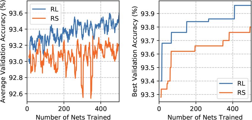
The progress of the architecture search process is reported
cells have a similar number of parameters as the normal
in Figure 8, where we can observe similar trends as the ones
3 × 3 convolution layer.
in Figure 7. Moreover, we find that the advantage of RL
over RS is larger in this case (RL achieves 1.54% better
B.2. Skip Node Connection and BN layer
validation accuracy than RS). After 300 epochs training on
CIFAR-10, the best RL identified cell reaches 3.93% test Inspired by PyramidNets (Han et al., 2017) that add an ad-
error with 11.5M parameters, which is better than 4.44% ditional batch normalization (BN) (Ioffe & Szegedy, 2015)
given by the best random cell with 10.0M parameters, but layer at the end of each residual unit, which can enable the
is far worse than 3.14% given by TreeCell-A with 5.7M network to determine whether the corresponding residual
parameters. unit is useful and has shown to improve the capacity of the
network architecture. Analogously, in a tree-structured cell,
we insert a skip connection for each child (denoted as Nic (·))
Table 3. Start point network with identity mappings on CIFAR-10. of the root node, and merge the outputs of the child node
Model architecture Feature map size Output channels and its corresponding skip connection via add. Additional,
3 × 3 Conv 32 × 32 48 the output of the child node goes through a BN layer before
[identity mapping] ×4 32 × 32 48 it is merged. As such the output of the child node Nic (·)
1 × 1 Conv 32 × 32 96
3 × 3 average pooling, stride 2 16 × 16 96 with input feature map x is given as:
[identity mapping] ×4 16 × 16 96
1 × 1 Conv 16 × 16 192 Oi = add(x, BN (Nic (x))). (4)
3 × 3 average pooling, stride 2 8×8 192
[identity mapping] ×4 8×8 192
8 × 8 global average pooling 1×1 192 In this way, intuitively, each unit with tree-structured cell
10-dim fully-connected, softmax can at least go back to the original unit if the cell is not
helpful here.
C. Detailed Structure of TreeCell-B
x Leaf
Replication
Add
GroupConv GroupConv
3x3 3x3
Replication Replication
Add Add
Conv Sep Avg Sep
1x1 7x7 3x3 7x7
Figure 8. Progress of the architecture search process starting from
scratch (a chain of identity maps) on CIFAR-10. Replication
Add
Sep Avg Sep Conv Avg
5x5 3x3 7x7 1x1 3x3
B. Details of Architecture Space
We find the following 2 tricks effective for reaching good
performances with the tree-structured architecture space in Figure 9. Detailed structure of TreeCell-B.
our experiments.Path-Level Network Transformation for Efficient Architecture Search
D. Meta-Controller Training Procedure
Algorithm 1 Path-Level Efficient Architecture Search
Input: base network baseN et, training set trainSet, validation
set valSet, batch size B, maximum number of networks M
1: trained = 0 // Number of trained networks
2: Pnets = [] // Store results of trained networks
3: randomly initialize the meta-controller C
4: Gc = [] // Store gradients to be applied to C
5: while trained < M do
6: meta-controller C samples a tree-structured cell
7: if cell in Pnets then
8: get the validation accuracy accv of cell from Pnets
9: else
10: model = train(trans(baseN et, cell), trainSet)
11: accv = evel(model, valSet)
12: add (cell, accv ) to Pnets
13: trained = trained + 1
14: end if
15: compute gradients according to (cell, accv ) and add to Gc
16: if len(Gc ) == B then
17: update C according to Gc
18: Gc = []
19: end if
20: end whileYou can also read