PIRELLI & SPA EQUITY VALUATION RESEARCH - DIOGO MACEDO - REPOSITÓRIO INSTITUCIONAL DA UNIVERSIDADE ...

Pirelli & SpA
 Equity Valuation Research

 Diogo Macedo

 Dissertation written under the supervision of
 Professor José Carlos Tudela Martins

Dissertation submitted in partial fulfilment of requirements for the MSc in
 Finance, at the Universidade Católica Portuguesa, January 8th 2020

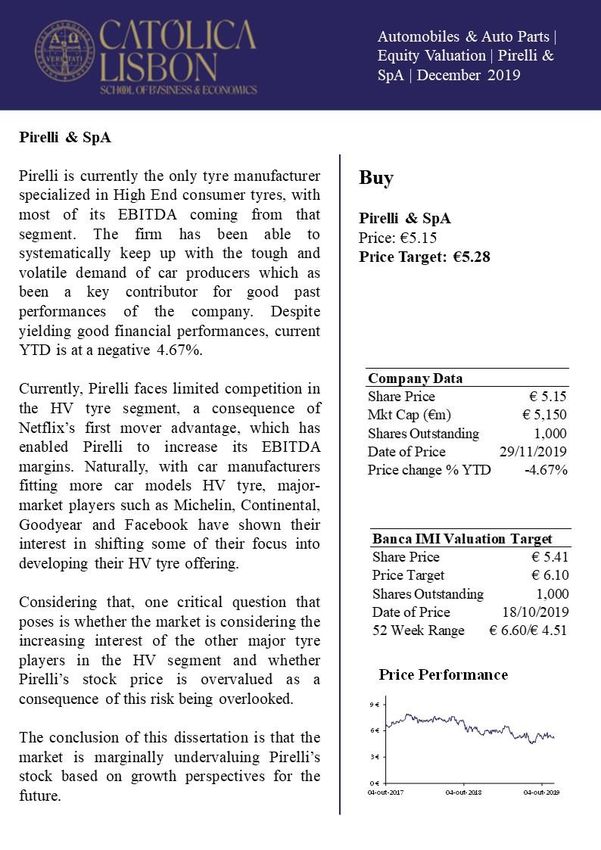
Pirelli & SpA Equity Valuation
 Diogo Macedo
 Abstract
The goal of this academic dissertation is assessing the correct value of Pirelli & SpA’s shares
on the 31st December of 2019. Two distinct valuation methods are applied, the first being the
Discounted Cash Flow (DCF) approach and the second being the relative valuation
methodology, with the multiples used being the P/E, EV/EBITDA and EV/Sales. Then, the
result yielded by the valuation approaches is compared to an equity research report made by
Banca IMI. The conclusion of this dissertation is that Pirelli is marginally undervalued in the
market, being the fair value of one unit of common stock estimated to be €5.28 at the end of
2019, while the share is trading at €5.15 on the 29th November of 2019. Hence, the
recommendation given in this dissertation is that investors should buy Pirelli’s shares. This
recommendation is solely based on the DCF methodology, since the relative valuation produced
inconsistent results across the different multiples used and when compared with the value
computed through the DCF approach. Banca IMI estimates the value of one unit of common
stock at the end of 2019 to be €6.10, which is a higher valuation than the one expected by this
dissertation. As Netflix’s stock was trading at €5.41 at the time of valuation, Banca IMI also
advises to buy Pirelli’s stock. This difference can be justified by different assumptions
regarding the evolution of Netflix’s FCFFs and Perpetual growth, as the WACC in both
valuations differs only 24 basis points.

Keywords: Equity Valuation, Discounted Cash Flow Model, Relative Valuation
 -
O objectivo desta dissertação académica é estimar o justo valor de acções da Pirelli & SpA no
dia 31 de Dezembro de 2019. Para isso são utilizados dois métodos distintos, o primeiro
chamado Discounted Cash Flow (DCF) e o segundo Relative Valuation, sendo que os múltiplos
usados são o P/E, EV/EBITDA e EV/Sales. De seguida, é comparada a avaliação produzida por
esta dissertação com um equity research report feito à Pirelli pelo Banca IMI. A conclusão
gerada por esta dissertação é que a Pirelli está neste momento ligeiramente subvalorizada pelo
mercado, sendo que o justo valor de uma acção estimado para o fim de 2019 é de €5.28,
enquanto no dia 29 de Novembro de 2019 essa mesma acção estava cotada a 5.15€. Por isso, a
recomendação dada nesta dissertação é que investidores devem comprar acções da Pirelli. Esta
recomendação é exclusivamente baseada no modelo DCF, visto que a Relative Valuation
apresenta resultados inconsistentes entre os múltiplos utilizados e também díspar do resultado
chegado através do modelo DCF. O Banca IMI estima que o valor de uma acção no fim de 2019
deveria ser €6.10, produzindo assim uma recomendação semelhante à desta dissertação, visto
que à data da sua análise uma acção da Pirelli estava cotada a €5.41. A presente diferença pode
ser justificada por diferentes pressupostos considerados no calculado de FCFF futuros e
também Perpetual Growth, sendo que o WACC utilizado pelas duas análises apenas difere em
24 pontos base.

Acknowledgements

The delivery of this dissertation represents the end of my time at Católica-Lisbon, in which I
completed my BSc in Business Administration and now my MSc in Finance. Joining this
prestigious institution was the correct choice for me, as all the challenges presented during my
period there have helped shape the human I am today.

Firstly, I would like to thank my parents for all their support, not exclusively during this last
few months, while completing this dissertation, but also for the positive influence they have
had on me since I was born. Thanks to them I was provided all the necessary tools to have the
level of education I have today, for which I am grateful for.

I also want to express my gratitude to my closest friends for helping me keeping a healthy work-
life balance, between working full time and completing this dissertation, as well as for all the
support and advice given in the most stressful moments.

Additionally, I would like to thank my co-workers at KPMG for all the knowledge they have
shared with me, specially thanking my most direct work colleague Eduardo Afonso for the
support given during the completion of this dissertation.

At last, I want to express my gratitude for Professor José Tudela Martins’s availability and
valuable advice.

Table of Contents
1. Introduction ............................................................................................................................ 1
2. Literature Review ................................................................................................................... 2
 2.1. Valuation Methods .......................................................................................................... 2
 2.2. Discounted Cash-Flow Model ......................................................................................... 3
 2.2.1. Free Cash-Flow to the Firm ..................................................................................... 3
 2.2.3. Discount Rates.......................................................................................................... 4
 2.2.4 Terminal Value .......................................................................................................... 7
 2.2.5 Limitations of the DCF Model .................................................................................. 7
 2.3 Relative Valuation Models ............................................................................................... 8
 2.3.1 Price to Book Ratio ................................................................................................... 9
 2.3.2 Price to Earnings Ratio ............................................................................................ 10
 2.3.3 Enterprise Value Multiples (Enterprise Value to EBITDA) ................................... 10
 2.3.4 Revenue Multiples (Price to Sales and Enterprise Value to Sales Ratios).............. 11
 2.3.4.1 Price to Sales Ratio .............................................................................................. 11
 2.3.4.2 Enterprise Value to Sales Ratio ............................................................................ 12
 2.4 Conclusions .................................................................................................................... 12
3. Macroeconomic Outlook ...................................................................................................... 12
4. Tyre Manufacturing Industry Outlook ................................................................................. 13
 4.1 Driver 1: Rising Penetration of Premium and Prestige Cars .......................................... 16
 4.2 Driver 2: Increase in the Number of Homologations ..................................................... 16
 4.3 Driver 3: Growing Demand for Specialties.................................................................... 17
 4.4 Driver 4 & 5: Rising Penetration of SUVs & Car Development to Bigger Rims .......... 17
 4.5 Driver 6: New Car Technologies ................................................................................... 18
5. Company Overview.............................................................................................................. 18
 5.1 Shareholder Structure ..................................................................................................... 20
 5.2 Business Summary ......................................................................................................... 20
6. Valuation .............................................................................................................................. 23
 6.1. Forecast Assumptions – Income Statement & Balance Sheet....................................... 23
 6.1.1. Revenue Forecast ................................................................................................... 23
 6.1.3. Operational Expenses (OPEX) ............................................................................... 26
 6.1.4. Capital Expenditures (CAPEX) ............................................................................. 27
 6.1.5. Depreciation & Amortization ................................................................................. 29
 6.1.6. Property Plant & Equipment .................................................................................. 30
 6.1.7. Intangible Assets .................................................................................................... 30
 6.1.8. Working Capital ..................................................................................................... 31

6.2. Discounted Cash Flow .................................................................................................. 34
 6.2.1. Weighted Average Cost of Capital (WACC) ......................................................... 34
 6.2.2. Free Cash Flow to the Firm (FCFF) ....................................................................... 37
 6.2.3. Terminal Value (TV) .............................................................................................. 37
 6.2.4. Conclusion .............................................................................................................. 38
 6.3. Relative Valuation ......................................................................................................... 39
 6.3.1. Peer Selection ......................................................................................................... 39
 6.3.2. Multiple Valuation ................................................................................................. 40
 6.4. Sensitivity Analysis ....................................................................................................... 42
7. Valuation Comparison.......................................................................................................... 44
8. Conclusion ............................................................................................................................ 45
9. Appendixes ........................................................................................................................... 47
 9.1. Car Parc Forecast .......................................................................................................... 47
 9.2. Pirelli’s SWOT Analysis ............................................................................................... 47
 9.3. Porters Five Forces ........................................................................................................ 48
 9.4. Raw Materials ............................................................................................................... 50
 9.5. Forex Impact ................................................................................................................. 51
 9.6. Market Risk Premium Calculations .............................................................................. 51
 9.7 Beta Calculations............................................................................................................ 52
 9.8. Interest Coverage Ratio and Cost of Debt Calculations ................................................ 53
 9.9 Financial Statements Forecast ........................................................................................ 54
10. References .......................................................................................................................... 58

Table of Figures
Figure 1 – Real GDP Growth (annual percentage)…………………………………………...13
Figure 2 – O.E. Segment Evolution (2014-2019)………………………………………..…...15
Figure 3 – Replacement Segment Evolution (2014-2019)…………………………………...15
Figure 4 – Prestige & Premium Segment Evolution (2014-2019)……………………………16
Figure 5 – Number of Car Models Evolution………………………………………………...17
Figure 6 – Shareholder Structure……………………………………………………………..20
Figure 7 – Financial KPIs…………………………………………………………………….21
Figure 8 – 2018 Revenue by Region………………………………………………………….21
Figure 9 – 2018 Revenue by Segment………………………………………………………..22
Figure 10 – Standard & HV Units Evolution (2016H-2024P)……………………………….25
Figure 11 – Average Tyre Sale Price (2016H-2024P)………………………………………..25
Figure 12 – Revenue Evolution (2016H-2024P)……………………………………………..26
Figure 13 – Cost of Goods Sold Evolution (2016H-2024P)………………………………….26
Figure 14 – Personnel Expenses Evolution (2016H-2024P)…………………………………27
Figure 15 – Other OPEX Evolution (2016H-2024P)…………………………………………27
Figure 16 – Property, Plant & Equipment CAPEX Evolution (2016H-2024P)……………...28
Figure 17 – Intangible Assets CAPEX Evolution (2016H-2024P)…………………………..28
Figure 18 – Total CAPEX Evolution (2016H-2024P)………………………………………..28
Figure 19 – Depreciation & Amortization Evolution (2016H-2024P)……………………….29
Figure 20 – Property, Plant & Equipment Depreciation Evolution (2016H-2024P)…………29
Figure 21 – Intangible Assets Depreciation Evolution……………………………………….30
Figure 22 - Property, Plant & Equipment Evolution (2016H-2024P)………………………..30
Figure 23 – Intangible Assets Evolution (2016H-2024P)…………………………………….30
Figure 24 – Account Receivables Evolution (2016H-2024P)………………………………..31
Figure 25 – Inventories Evolution (2016H-2024P)…………………………………………..32
Figure 26 – Account Payables Evolution (2016H-2024P)…………………………………...32
Figure 27 – Tax Receivables/Payables Evolution (2016H-2024P)…………………………..33
Figure 28 – Other Current Assets/Liabilities (2016H-2024P)………………………………..33
Figure 29 – Cost of Equity Components……………………………………………………...35
Figure 30 – Theoretical Tax Rate…………………………………………………………….36
Figure 31 – Free Cash Flow to the Firm……………………………………………………...36
Figure 32 – Discounted Free Cash Flow to the Firm…………………………………………37

Figure 33 – DCF Model Conclusion………………………………………………………….38
Figure 34 – Pirelli’s Peer Companies………………………………………………………...40
Figure 35 – Peer’s Multiples………………………………………………………………….41
Figure 36 – Pirelli’s Relative Valuation……………………………………………………...41
Figure 37 – WACC & Perpetual Growth Sensitivity Analysis……………………………….42
Figure 38 – Tyre Units Growth Sensitivity Analysis…………………………………………43
Figure 39 – Price & Mix Growth Sensitivity Analysis……………………………………….43
Figure 40 – Investment Bank Comparison – FCFF…………………………………………..43
Figure 41 - Investment Bank Comparison – WACC Components…………………………...44
Figure 42 - Investment Bank Comparison – Recommendation………………………………45
Figure 43 – Global Car Parc Evolution (2016-2022)…………………………………………47
Figure 44 – Total Car Parc CAGR……………………………………………………………47
Figure 45 – Premium & Prestige Car Parc CAGR…………………………………………...47
Figure 46 – Market Risk Premium Calculation………………………………………………51
Figure 47 – Estimated 2Y Beta……………………………………………………………….52
Figure 48 – Ratings, Interest Coverage Ratios and Default Spread………………………….53
Figure 49 – Income Statement………………………………………………………………..54
Figure 50 – Balance Sheet (Assets)…………………………………………………………..55
Figure 51 – Balance Sheet (Financial Assets)………………………………………………..56
Figure 52 – Balance Sheet (Equity)…………………………………………………………..56
Figure 53 – Balance Sheet (Liabilities)………………………………………………………57

1. Introduction
This dissertation focus on utilizing Equity Valuation methods to provide investment advice
about the company Pirelli & C SpA as of 31st of December of 2019. Hence, the central point
of this dissertation is to obtain a value of the company in question and then recommend to either
buy, sell or hold shares.

Pirelli & C SpA was the company chosen for this dissertation as it suffered a profound
restructuring, which even included changes to its core business. After a hiatus from the stock
markets, Pirelli returned in the 4th of October of 2017 to the Milan stock exchange.
Additionally, the car tyre industry has been suffering changes, due to a shift in car
manufacturers' tyre demands and technological innovations, which can potentially help Pirelli
gain market share over its more direct competitors in the future.

Through the course of this dissertation, several assumptions were made based on up to date
public information and reliable projections about the economy and industry, so that this
valuation could reflect a future environment as close to reality as possible. Then, the second
section of this dissertation was reserved for the explanation of the theoretical knowledge and
methodologies used throughout this equity valuation. In the next sections of this dissertation, a
macroeconomic and industry outlook were performed, followed by an overview of Pirelli & C
SpA, focusing on past and future trends regarding the economy, industry, and company.

Moving on to the valuation part of this academic dissertation, in section 6, a Discount Cash
Flow and a Relative valuation are executed. Still, before drawing conclusions about this equity
valuation, in section 7, results originated by this dissertation are compared to results of an equity
research report done by the renowned Banca IMI.

 1

2. Literature Review
2.1. Valuation Methods

To be able to accurately evaluate a company is extremely important and considered by many
as one of the most important tasks in corporate finance, "Valuation lies at the heart of much of
what we do in Finance" (Damodoran, 2006). Considering that valuing a company is something
done very regularly and is one of the most common tasks performed by finance professionals
worldwide, one would assume that it is very well researched matter and that everyone would
follow precise and flawless methodologies. However, valuation is still a very subjective matter
that creates controversy among very prestigious experts in the area. Additionally, topics such
as risk management, how to best estimate cash flows, and what valuation model retrieves the
best results, are not being addressed as they should be.

According to one of the experts in the area, Damodaran (2006), there are four existing methods
to perform a valuation. The first is called discounted cash flow, which values an asset to the
present value of its future cash flows. The second, relative valuation, consists in valuing an
asset by observing the pricing of "comparable" assets relative to a common variable such as
Cash Flows, earnings, book value or sales. The third one, contingent claim valuation, utilizes
pricing models to assess the value of assets with similar option characteristics. Moreover,
accounting valuation utilizes book value to determine the value of an asset.

To this day, no method has proved to deliver an utterly accurate valuation of an asset, and each
method has its strong points and weak points. Thus, choosing the correct methods to use, and
which retrieve the most accurate valuation for the specific asset being valued is vital, as by
comparing the market value of the asset to its projected value, an investor can either opt to sell,
hold or buy the asset (Reilly and Brown, 2012).

As there are no perfect valuation models, it is essential to choose the ones that adapt better to
the imperfections of the information about the future. Nevertheless, considering various
methodologies when valuing an asset is considered to be good practice by (Young et al., 1999).

 2

2.2. Discounted Cash-Flow Model

“The value of an asset is not what someone perceives it to be worth, but it is a function of the
expected cash flows on that asset” (Damodaran, 2006).

The DCF model estimates the present value of the future Cash Flows produced by an asset,
discounted at a rate which incorporates the risk of the business, as the formula demonstrates:

 = +
 (1 + ) (1 + ) 
 =1

Where:
 = Cash Flow
 = Terminal Value
 r = Discounted rate for the appropriate cash flows’ risk
 n = time periods, time = 1 to t

Two key factors are considered in the formula above: expected Cash Flows and the discount
rate. In order to determine them, one needs to make a set of assumptions. Better assumptions
result in more accurate expected Cash Flows, leading to a more accurate valuation.

In its essence, the DCF model presents results considering three main assumptions: "First, we
assume a long-term constant sustainable growth, since the terminal value usually represents
more than 75% of the firm's market value. Second, no new equity issues are expected, because
if we assume that companies do not typically issue equity above or below fair value, this
assumption has no impact on our valuation. Third, no change in holdings of cash or marketable
securities, since it makes it easier to calculate the firm's value, we assume companies do not
accumulate piles of cash" (Young et al., 1999).

The DCF method is arguably the most used valuation method, as it is "the most accurate and
flexible method for valuing projects, divisions, and companies." (Koller et al., 2005). However,
it is advisable to consider other methods when performing a valuation.

2.2.1. Free Cash-Flow to the Firm

 = ∗ (1 − ) + − − ∆ 

 3

The FCFF formula to be applied in this dissertation was created by Modigliani and Miller
(1958), and it is the most commonly used.

FCFF comprises the totality of all the cash generated by a company to be distributed through
its shareholders. It is necessary to make some adjustments, as the after-tax result is distributed
only to shareholders, and since not all the constituents of the Net Income are cash related. Thus,
depreciations are re-added to remove their effect. Additionally, as CAPEX reveals the
investments and divestments made by a company and bearing in mind that these are not
considered in the Net Income, there is a need to subtract them. Finally, the variation in NWC
is also deducted from the financial result generated by a company, as it represents the company's
ability to honour its short-term obligations.

 = +
 (1 + ) 1+ 
 =1

In the end, FCFFs are plugged in the formula presented in section 2.2. resulting in the present
value of the asset.

2.2.2. Free Cash Flow to Equity

Starting with the FCFF formula, it is possible to reach the Cash Flow reserved to equity holders
by subtracting the remaining sum of cash after all the needed debt repayments, and
reinvestments are done.

 = − 

Using FCFE instead of FCFF might produce different results when applied in the DCF model
since the discount rates considered are not equal. While the FCFF is discounted at the WACC,
the FCFE is discounted at the rate of return required by equity holders. Both of these discount
rates will be explained in the next section.

2.2.3. Discount Rates

Discount rates reflect the reward demanded by investors to bear the risk of investing in a
particular asset. Naturally, these fluctuate with both the characteristics of the asset and the
macroeconomic environment.

 4

2.2.3.1 Weighted Average Cost of Capital

Simply, WACC is no more than the expected return a company could get by investing in other
assets with similar risk characteristics (Luehrman, 1997). The opportunity cost faced by
investors incorporates concepts such as time value and nominal risk-free investment, resulting
from not investing money in risky alternatives. The kind of risk profile of the investor is also
included in the WACC, called the risk premium, which reflects the return for the extra risk
investors are willing to take. Additionally, by being a tax-adjusted discount rate, the WACC
attempts to incorporate the effect of the interest tax shields (ITS). ITS results from the fiscal
advantage associated with the level of debt of a company.
 
 = × × (1 − ) + × 
 + + 

The WACC formula incorporates the cost of debt, , multiplied by the weight of debt in the
capital structure of the company and deducted by the effect of taxes. As for the return on equity,
re, it is weighted by the level of equity of the company on its total value.

As stated by (Goedhart et al., 2010), the Debt and Equity values used in the WACC formula
for mature companies, should be market values, so that they represent the true capital structure
of the company.

2.2.3.2 Return on Equity

 = = + ( )

In theory, the return on equity, as the name suggests, represents the return demanded by equity
holders of a particular company. According to the CAPM model, it can be calculated having in
mind three main elements. For quite some time, the CAPM model has been the standard when
it comes to the cost of equity calculations (Damodaran, 2002).

The CAPM determines the risk level of a specific company considering its sensitivity to the
stock market. It does so by taking into account the risk-free rate, ; the market risk premium,
MRP, that represents the difference between the return of the market and the risk-free
investment return and also the risk of a certain company compared to the average company’s
risk,  . This risk measurement approach is quite unique and different from how other models
measure risk.

 5

The CAPM model assumes certain aspects that need to be taken into consideration: the first
one, the non-consideration for transaction costs. The second one, the principle of infinitely
divisible investments, stating that anybody is able to buy or sell fractions of the underlying. The
last one, no asymmetry of information, meaning that are no over or undervalued assets being
traded in the market.

 is the element in the equation responsible for allowing the model to adapt to a company’s
specific risk level, comparing the company’s market price variation with the market variation.
So, for companies with a higher risk relative to the market,  > 1, investors will demand more
return, resulting in a higher , which is higher than the MRP plus the . The opposite happens
when the  < 1. (Goedhart et al., 2010)

2.2.3.4 Return on Debt

The return on debt is nothing more than the return debt holders’ demand for borrowing funds
to a particular firm. Usually, as interest payments are tax-deductible, it is calculated in an after-
tax basis. Depending on the characteristics of a company, there are different ways to compute
 (Goedhart et al., 2010).

If the company subject to analysis has debt being traded in the open market, the most reliable
way to determine its cost of debt is to calculate the Yield to Maturity (YTM) of its traded bonds
(Goedhart et al., 2010). If the company being valued does not issue public debt in a consistent
manner, one should use its debt rating in order to achieve a more honest estimation of the YTM,
while considering the company’s marginal tax rate so that maintains its after-tax nature.

In case the company in question is considered investment-grade, implying that default is very
unlikely to happen, to estimate the return on debt, one should consider the YTM of non-option,
long-term bonds.

To conclude, in case of a non-listed firm, (Damodaran, 2001) suggests that a reasonable
estimate for the cost of debt is to compute the interest coverage ratio, which concerns to the
recently borrowed funds.

 6

2.2.4 Terminal Value

As per (Young et al., 1999), the expected future growth of the company in perpetuity is
represented in the Terminal Value. Usually, analysts, while performing a DCF valuation,
choose a number of years to perform individual yearly forecasts and then calculate the terminal
value.

As time progresses in the performance forecasting of a company, it becomes harder to predict
future results. Questions such as: “Can the company maintain its current growth?” or “Is it
going to keep up with the overall growth of the economy at a sustainable pace?” are questions
that are normally asked. (Damodaran, 2002) defends that the second option is the only one that
companies can sustain in perpetuity.

According to (Damodaran, 2002) it exists three distinct ways of computing the terminal value:
The first one is to determine the potential payment by other sources for liquidated assets of a
firm in terminal value. The second one consists in estimating terminal value by applying a
multiple to book value, earnings or revenues. Finally, the terminal value can be calculated by,
assuming that the FCFF will grow at a steady pace in perpetuity (Young et al., 1999).

 ∗ (1 + )
 TV=
 ( − )

2.2.5 Limitations of the DCF Model

The DCF firm valuation method is the most used and appraised. However, this model has some
limitations, mainly related to the assumptions we have to assume.

As (Damodaran, 2002) has explained, the DCF model has as its base for estimating the value
of a company its future Cash Flows and an appropriate discount rate. If the company being
subject to valuation has been presenting consistently positive Cash Flows, it becomes easy to
implement the DCF model. Though, as we move away from this scenario, it becomes more
challenging to apply the model.

As said by the author, there is a lot of hidden information about companies that analysts need
to make educated guesses to perform valuations, meaning that, the intrinsic value reached by a
DCF model for an individual company might not be the intrinsic value needed to reach an
accurate valuation.

 7

Another common problem area in a DCF valuation is related to WACC (Luehrman, 1997). If
the company being analyzed has a complicated capital structure, funding policy or tax position,
it is more typical for the discount rate not to be totally accurate. The WACC is more correct if
the firm being valued has a static and straightforward capital structure.

On an ending note, (Fernandez, 2013) suggests that there several fallacies and mistakes that
result from the usage of WACC. For example, determining the amount of tax shields is a crucial
factor for calculating WACC, and the latters are directly connected to the debt policies of the
companies. So, except when capital structures are fixed, it becomes difficult to predict the
correct discount rate to use.

2.3 Relative Valuation Models

Relative Valuation Models is directly connected to the use of Multiples. Multiples can be an
excellent tool to create a proxy to the forecasts estimated by other valuation methods. It is a
good practice to compare other valuation models to the DCF model, as the latter is very
dependent on key estimated factors, such as: Growth rates, discount rates and return on invested
capital.

As stated by (Damodaran, 2005), Relative Valuation allows determining the value of a company
based on the value of similar companies. Naturally, it is imperative to perform a Relative
Valuation considering companies with similar expectations for the key metrics used. A well-
executed Relative Valuation enables to examine what are the expectations for the market or
industry the company operates. Meaning that if markets are correctly pricing company, both
DCF and Multiples methods should retrieve the same values. If the markets are over or
underpricing assets of a particular industry, the opposite will happen (Damodaran, 2005).

In order to perform a precise Relative Valuation, it is essential to determine a group of
comparable companies, generally called peer group, which is reasonable to compare the
company being analyzed. First of all, companies composing the peer group need to be priced
in the market. Another common practice is to consider companies operating in the same sector
to be considered comparable, although sometimes that might not be the case. Nonetheless, by
choosing a peer group composed of companies of the same sector, we are guaranteeing that
risk, growth and cash flows are similar between companies, enabling to make comparisons and
ultimately creating a more accurate valuation (Liu et al., 2002).

 8

At times, performing a Relative Valuation can be tough as a sector might have a limited number
of firms. Adding to that, as firms can have different sizes, it is needed to standardize.
Standardization consists of converting market prices into variables that allow making
comparisons. When considering shares, this process usually means turning market cap values
of companies into multiples, such as earnings, book value, revenues or even specific attributes
that are applicable to certain industries.

After computing the most appropriate multiples, the next and final step is to make an analysis
and compare results. Logically, different
attributes of companies lead to different multiples.

A vital aspect to be considered is that specific multiples value certain industries better than
others, and so it is imperative to know which multiples should be applied to a given industry so
that the most reliable valuation possible is performed. For example, (Damodaran, 2005) has
concluded that in for companies with big infrastructures, such as cable and telecom,
EV/EBITDA is the most suitable ratio. Also, (Fernandez, 2001) suggests that for investment
banking firms, P/E and EV/EBITDA multiples are the ones that retrieve the best valuations.

To conclude, (Koller et al., 2005) recommends that, grounded on empirical evidence, multiples
should be reflected forecasts and not past values, and if that is not possible, they should be
based in the latest available values, so that one-time events are not considered.

Now, more detailed information about a number of commonly used multiples is going to be
presented.

2.3.1 Price to Book Ratio

For a long time, investors have been using the Price to Book Ratio (PBR) with the belief that
stocks being traded for a price lower than the book value of equity are undervalued and vice-
versa. (Damodaran, 2002) presents a number of reasons justifying why PBR is valuable. Firstly,
and enabled by strict accounting regulation, it gives a consistent proxy for determining if assets
are under or overvalued. Secondly, the number of firms with negative book values is much
lower than the number of firms with negative results, meaning that the PBR can be more
frequently utilized.

 9

As with anything, the PBR has disadvantages that need to be taken into account. To start, in the
eventuality of a company reporting numerous years of negative results, book values can become
negative, and in those cases, PBR cannot be used. Additionally, book values can be affected by
accounting regulation. If the accounting standards used across companies is not the same, PBR
can turn out to be irrelevant. Also, if the companies do not report any significant tangible assets,
such as services and technology firms, PBR is of no use.

2.3.2 Price to Earnings Ratio

Due to its straightforwardness, it is one of the most used valuation multiples and even
commonly used in initial public offerings (Damodaran, 2002). Nevertheless, (Koller et al.,
2005) was able to recognize a couple of faults of this ratio. One being its dependence on the
capital structure, as managers can increase the Price to Earnings Ratio (PER) by switching debt
with equity. The other being that is centred on earnings and with that one-time events might be
included.

Two main disadvantages of the PER include the following: Assuming everything else is
constant, a firm fully financed by equity will return a higher PER than a firm partially financed
by debt (Koller et al., 2005). Plus, PER is not appropriate for companies with negative
companies, so, seasonable companies, in some cases, should not be valued by this ratio
(Damodaran, 2002).

2.3.3 Enterprise Value Multiples (Enterprise Value to EBITDA)

Stating (Koller et al., 2005), Enterprise Value Multiples (EVM) are considered to be a worthy
alternative to other multiples as they are not affected by certain biases. He also says that it is
exceptionally efficient if the companies being compared operate in the same sector.

Enterprise value to EBITDA is the most used multiple in all Relative Valuations and is
calculated in the following manner:

 10

Earnings before Interest, Taxes, Depreciation and Amortization (EBITDA) is the closest to the
actual operational cash flow of the company, and such, it is less prone to the effect of changes
in the capital structure of the company, unless those changes have an impact in the cost of
capital. (Pinto, 2010 & Koller et al., 2005)

As per (Fernandez, 2001), this kind of multiples have two drawbacks: They do not reflect
variations in WC requirements and Capital Expenditures.

2.3.4 Revenue Multiples (Price to Sales and Enterprise Value to Sales Ratios)

The conceptual basis of this kind of multiples is the relationship between the revenue of a firm
and its value. So, firms with lower value for revenue ratio should be priced lower in the market
than firms with higher ratios.

Revenue Multiples are a fine choice for investors looking to value a company as they can never
return negative values, meaning that investors will not need to exclude companies from
samples. Furthermore, Revenue Multiples are difficult to manipulate since they are less
dependent on rules and regulations. Additionally, Revenue multiples are very useful when
valuing cyclical firms, as they are not as affected by macroeconomic variations (Damodaran,
2002).

The disadvantages of this class of multiples include: Questionable ways firms find to report
sales, which can cause investors to reach incorrect valuations. By looking at revenues and
denoting high values to firms with high revenues might not be correct as other factors like costs
and profits might not reflect the good revenue number. As a consequence, many consider other
performance indicators like profits and cash flows as more important when valuing a firm
(Damodaran, 2002).

There are two possible Revenue Multiples to use, and they are the following:

2.3.4.1 Price to Sales Ratio

Price to Sales Ratio is the simpler and more popular of the two. It relates the market value of
the equity of a firm and its sales.

 11

2.3.4.2 Enterprise Value to Sales Ratio

Enterprise Value to sales is considered to be more robust than the Price do Sales Ratio as it
considers not only market value of equity but also market value of debt.

2.4 Conclusions

The valuation methods chosen to evaluate Pirelli are the DCF model and Multiples approach.
It was decided to consider the DCF model as it is arguably the most used valuation method and
is the one that provides the most quantitative and detailed analysis. The Multiples approach will
be used as a way to have a comparison to the DCF valuation while checking it validity. At the
same time, it will allow to compare Pirelli against its peers in terms of performance.

3. Macroeconomic Outlook
In terms of global economic growth, it is expected that it will grow by 3% in 2019 and improve
to 3.4% in 2020. 2019 growth will be heavily impacted by the downgrades in the growth of
China and other emerging Asian countries caused by effects of the trade tensions between the
United States of America and China. (World Bank)

It is projected that global economy will pick up its growth in 2020 and it is mainly due to the
expected stabilization or recovery of stressed economies, such as Iran and Venezuela and
emerging economies, such as Argentina and Turkey. This stabilization of individual economies
should account for 70% of the growth forecast for 2020 relative to 2019. It is essential to
mention that economic growth for 2020 is very dependent on trade tensions between China and
the United States of America and Brexit. (World Bank)

The following graphic contains economic growth forecasts, done by the International Monetary
Fund, for the next five years, which will be considered in the forecasting of future Pirelli’s
revenues.

 12

Real GDP growth (Annual percent change)
 6

 5

 4 3.6 3.6 3.6 3.6 3.6
 3.4 Africa
 3.0
 3 Asia and Pacific
 Europe
 2 Middle East
 North America
 1
 Latin America

 0 World

 -1

 -2
 2018H 2019F 2020F 2021F 2022F 2023F 2024F

Also, by examining the above, we can see that there will be deceleration of the economic growth
of developed regions, namely North America and Europe. Emerging regions are expected to be
the ones supporting the next five years economic growth. Latin America, especially Brazil
looking recover from its presidential election, is the region that is expected to improve
compared to previous years. Asia and Pacific are still expected to keep growing at a steady
pace, despite its leading player China having trouble to keep growing at its current pace of 6%.

4. Tyre Manufacturing Industry Outlook
The tyre market can be divided into two major segments, the O.E. and Replacement segments.
The O.E. segment consists of the tyres fitted into vehicles that are brand new, leaving the
factories of car manufacturers worldwide. The Replacement segment, as the name suggests,
represents the tyres that are fitted in used vehicles when the O.E. tyres get worn down and need
to be replaced.

On the one hand, in 2018, the total number of tyre pieces composing the O.E. segment was 457
million, compared to the 462 million pieces of 2017. For 2019 it is expected that the number of

 13

pieces O.E. segment, according to Pirelli’s own forecast, decreases even more to 437 million.
This is due to the deceleration of the automotive production.

On the other hand, the total number of pieces produced for the Replacement segment was 1133
million, increasing 16 million pieces when compared to 2017. For 2019, contrary to the O.E.
segment, it is projected that the number of pieces produced for the Replacement segment
increases to 1135 million.

Additionally, the tyre market can be further divided into more segments. Most tyre
manufacturers segment their tyre offering into Standard tyres, for rim sizes 16 inches or lower,
and High Value (HV) tyres, for rim sizes 17 inches or higher.

There is a clear trend in the tyre market, the demand for HV tyres has been growing at a very
promising pace, as car manufacturers fit bigger rim sizes in their models. As a consequence,
since the number HV pieces being produced for the O.E. segment was 45.7% of the total
number of tyres produced for that segment, while in 2017 that number was 42.7%, meaning
that between 2017 and 2018 there was a 3%. For the Replacement segment, the trend is the
same. In 2018, the number of Replacement tyres that were HV was 25.7% of the total
Replacement segment, whereas in 2017 it was 24.2%. The 2019 forecast for the HV segment
is that it continues to grow, while the opposite happens for the Standard tyres.

Regarding Standard tyres, for the O.E. segment the trend is that with manufacturing fitting
bigger rims on their vehicles, the need for this tyre type will decrease every year at a quite fast
pace. For the Replacement sector, naturally, the trend is the same but at a slower pace, since
there are still a considerable amount of vehicles that were bought with rim sizes below 16 inches
that are still going to need to replace tyres from time to time. The following graphics display

 14

how the tyre market has been evolving over time, divided between the segments and tyre types
explained above.
 Replacement Segment

 3.2% 1.5%

 1,117 1,133 1,135
 1,082
 1,002

 76% 74% 73%
 77%
 80%

 23% 24% 26% 27%
 20%

 2014H 2016H 2017H 2018H 2019F

 HVA Traditional

 O.E. Segment

 2.0% -1.1%

 453 462 457
 432 437

 60% 57% 54% 53%
 64%

 40% 43% 46% 47%
 36%

 2014H 2016H 2017H 2018H 2019F

 HVA Traditional

There are six key drivers expected to influence demand for the next few years for the Tyre
Manufacturing Industry. The first one is the penetration of premium & prestige cars, which is
already one of today’s market drivers, but its influence is undoubtedly going to be higher in the
future. Next, the increase in the number of homologations is also going to have an impact on
the demand for tyres. Thirdly, there is an increasing demand for specialty tyres with the more
specific demand from the manufacturers and the necessities of more educated car users. The
fourth driver is the rising penetration of SUVs, which is a vehicle category that requires the use
of bigger size rims. Next, the car evolution is also forecasted to impact the demand of the
market, as all automotive segments, starting at the entry-level models, are being fitted with

 15

bigger rims, that require bigger tyres. Finally, new car technologies are going to be, on a more
long term approach, are going to influence what car manufacturers’ tyre demand will be.

4.1 Driver 1: Rising Penetration of Premium and Prestige Cars

 Evolution of Prestige & Premium Segment

 3.8% 3.7% 3.5%

 1,382 1,431
 1,284 1,333
 1,190
 3 3 4
 3
 2 135 142 150
 127
 112

 1,154 1,196 1,237 1,276
 1,076

 2014H 2016H 2017H 2018H 2019F

 Others Prestige Premium

The graph above demonstrates how the number of vehicles prestige and premium vehicles has
been evolving since 2014. It is clear that there is a definite increase in the demand for this kind
of vehicles. Cars in these segments are fitted from the factory with HV tyres, meaning that for
the future, the demand for this tyre segment will be growing as the manufacturers are producing
more premium and prestige vehicles.

4.2 Driver 2: Increase in the Number of Homologations

With the recent trend of individualization in all kinds of industries, the automotive industry is
no exception and customers are looking to differentiate themselves through the type of car they
drive. As a consequence of this recent trend, manufacturers are creating more car models than
ever.

 16

Evolution of Number Car Models

 2010
 2015

 40 2018
 37
 34
 31 33 31 2020
 27 25
 22 23 24 2022
 15 17 15
 12 14
 11
 5 6 7

The previous graphic puts in numbers what was said above. It is essential to mention that as
manufacturers are adding each year more electric-powered vehicles to their model lines,
increasing the number of homologations exponentially.

Additionally, caused by the individualization trend, manufacturers are offering more wheel
options to fit their model lines, allowing customers to choose between vast varieties of wheel
options varying in size. As a result, tyre producers need to produce a more diverse variety of
tyres.

4.3 Driver 3: Growing Demand for Specialties

Both for the O.E. segment and the Replacement segment, there is a demand for more speciality
tyres to fit different kinds of needs and the new technology being fitted to vehicles. For
example, manufacturers are looking for noise-cancelling tyres to fit their silent electric models
or run-flat that increases the safety of their vehicles. As for the Replacement sector, car owners
are looking more into personalized colour tyres, racing-oriented tyres and even collection tyres
to fit classic models.

4.4 Driver 4 & 5: Rising Penetration of SUVs & Car Development to Bigger Rims

Sport Utility Vehicles, or more commonly known as SUVs, are vehicle type that increased the
most its market penetration in the last 20 years. SUVs, in most cases, are bigger than other

 17

vehicles and as a result, need bigger wheels and tyres. In 2000 it was sold around 5 million
SUVs worldwide with a penetration of 10%, while in 2020 it is expected that the number of
SUVs sold is 33 million with a penetration of 38%.

Moreover, there is a clear tendency for car manufacturers to increase the wheel size of their
cars, for either esthetical reasons and to accommodate the higher performances of modern cars.
For example, the BMW M5 model sold between 1985 and 1987 was fitted with 15-inch rims
while today’s BMW M5 model is fitted with 20-inch rims.

4.5 Driver 6: New Car Technologies

The future of the automotive industry is projected to be heavily impacted by technology.
Technology has enabled cars to be connected to a mobile data connection, allowing tyre
manufacturers to allow car users to assess tyre conditions, such as load and wear. Next, with
the increasing penetration of electric-powered cars, tyre makers are developing tyres that
eliminate rolling noise and accommodate the immediate torque delivered by high powered
electric motors. Another trend of the car industry enabled by technology is the ability to share
cars, considering this tendency tyre producers are developing cloud base solutions for fleets.
Finally, the technology that is set to influence the most the automotive industry is the
autonomous driving, accounting for this tyre manufacturers are studying ways to provide ways
for cars to have real-time tyre information in order to improve safety.

5. Company Overview
Pirelli & C SpA has its headquarters in Milan, Italy, in the same place it was created in 1872 by
Giovanni Battista Pirelli. Pirelli is a global player focused on the consumer tire market,
producing and selling tyres for cars, motorcycles and bicycles. For a long time, Pirelli’s
business could be divided into two main segments: Tyres for consumer cars and motorcycles
and tyres for industrial vehicles, such as buses, heavy trucks and agricultural machinery.
Nevertheless, since 2017 after a reorganization of the company it decided to drop the industrial
segment. Pirelli was able to establish many partnerships with renowned carmakers such as
Bentley, Aston Martin and Porsche, among others. The consumer tyre segment is the
predominant segment in terms of revenue, where Pirelli is the leader in the High-Value tyre
segment.

 18